
PROBLEM
Figure 1 represents the structure of a swing. Study the axial stresses in the members of the structure for different loading conditions.
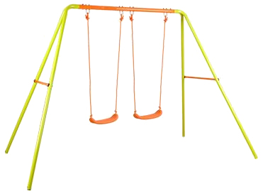
Figure 1. Swing.
All members have a circular cross section of diameter 35 mm and thickness 1.5 mm.
Figure 2 is the scheme of the swing with its dimensions.

Figure 2. Dimensions of the swing.
Table 1 indicates the mechanical properties for the steel.
Table 1. Mechanical properties for the steel.
| Laminated steel | |
| Esteel | 210 GPa |
| Sy steel | 275 MPa |
| νsteel | 0.3 |
Study the problem for three different loading conditions, as represented in Figure 3:
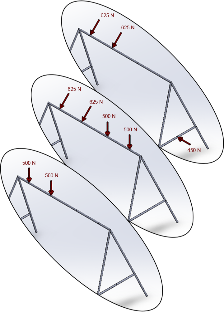
Figure 3. Loading conditions.
Obtain the deformation and the axial forces acting on the structure.
GEOMETRY OF THE MODEL
First, define the analysis type as "Structural".
Main Menu > Preferences
Then, select the element type "PIPE 2 node 288" (Figure 4):
Main Menu > Preprocessor > Element Type > Add/Edit/Delete
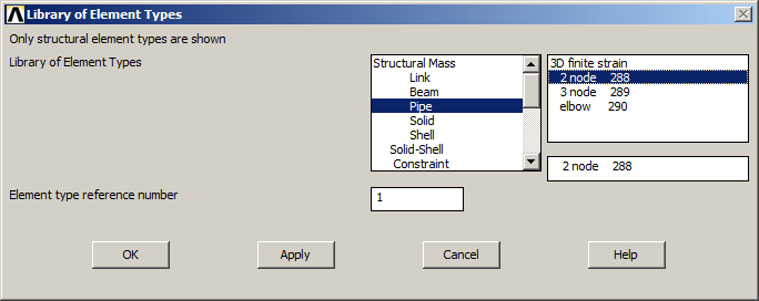
Figure 4. Element type.
Define the material properties according to Table 1.
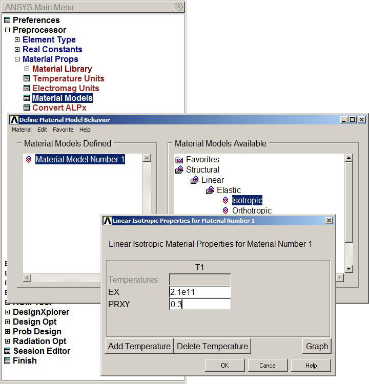
Figure 5. Material.
Define the geometric characteristics of the cross section:
Main Menu > Preprocessor > Sections > Pipe > Add
Input the parameters indicated in Figure 6.
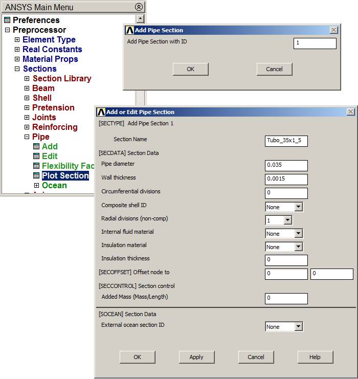
Figure 6. Input geometric characteristics for the PIPE section.
Plot the section (Figure 7):
Main Menu > Preprocessor > Sections > Pipe > Plot Section
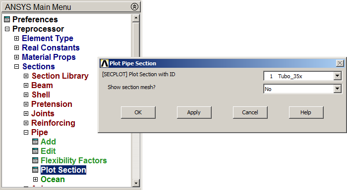
Figure 7. Plot Pipe Section.
Figure 8 represents the geometric characteristics of the pipe section.
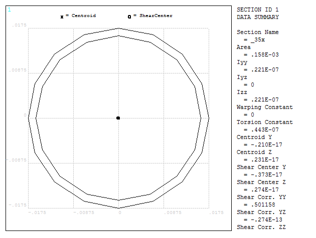
Figure 8. Geometric characteristics of the pipe section.
Now create the 14 keypoints from the coordinates indicated in Table 2.
Table 2. Coordinates for keypoints.
| Keypoint | X (m) | Y (m) | Z (m) |
| 1 | 0 | 0 | 0 |
| 2 | 0.08333 | 0.60 | 0.25 |
| 3 | 0.25 | 1.80 | 0.75 |
| 4 | 0.08333 | 0.60 | 1.25 |
| 5 | 0 | 0 | 1.5 |
| 6 | 0.55 | 1.80 | 0.75 |
| 7 | 1.15 | 1.80 | 0.75 |
| 8 | 1.85 | 1.80 | 0.75 |
| 9 | 2.45 | 1.80 | 0.75 |
| 10 | 2.75 | 1.80 | 0.75 |
| 11 | 2.91667 | 0.6 | 1.25 |
| 12 | 3 | 0 | 1.5 |
| 13 | 2.91667 | 0.60 | 0.25 |
| 14 | 3 | 0 | 0 |
Figure 9 represents the option "Create Keypoints in Active Coordinate System".
Main Menu > Preprocessor > Modeling > Create > Keypoints > In Active CS
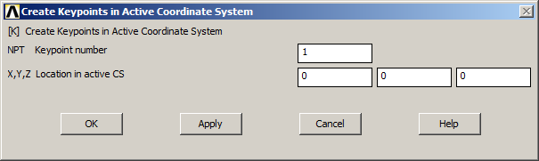
Figure 9. Input keypoints.
Select isometric view from the right menu (Figure 10).
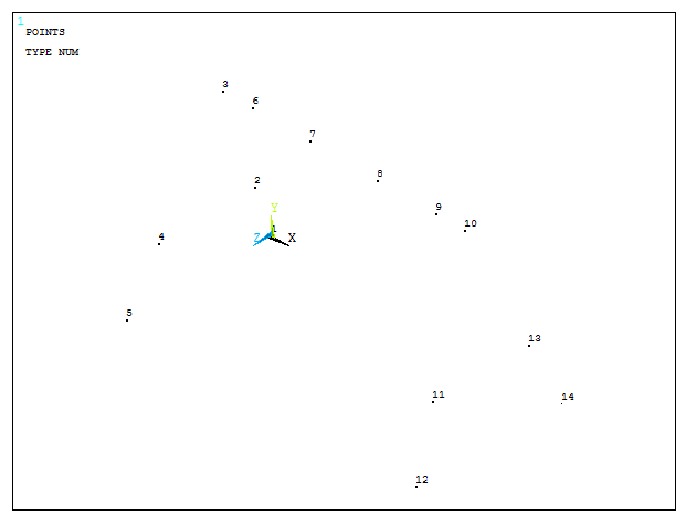
Figure 10. Graphic screen with the created keypoints.
After that, create the lines for the structure (Figure 11):
Main Menu > Preprocessor > Modeling > Create > Lines > Lines > Straight Line
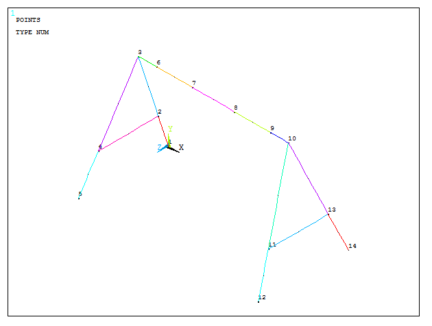
Figure 11. Structure with lines.
Main Menu > Preprocessor > Meshing > Size Cntrls > ManualSize > Lines > All Lines
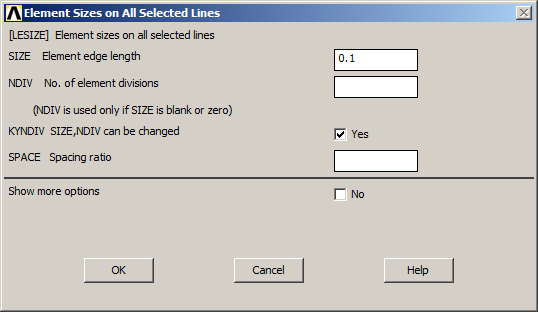
Figure 12. Size element for the mesh.
The size element is 0.1 meters. Figure 13 represents the division of the lines.
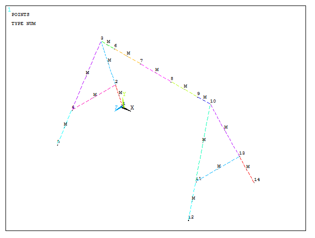
Figure 13. Graphic screen with the divided lines.
Now, mesh the lines (Figure 12):
Main Menu > Preprocessor > Meshing > Mesh > Lines
Click "Pick All". Figure 14 represents the model after the meshing process.
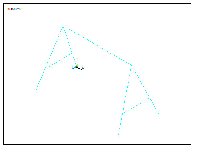
Figure 14. Meshed model.
Plot the scaled model with the option "Size and Shape" (Figure 15):
Utility Menu > PlotCtrls > Style > Size and Shape
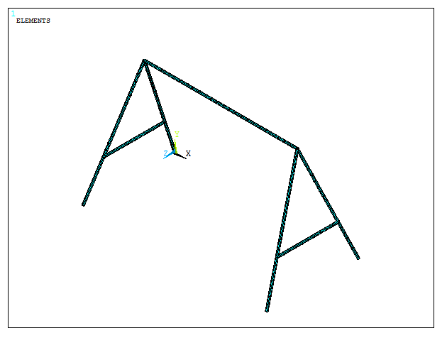
Figure 15. Scaled model.
LOADS AND BOUNDARY CONDITIONS
To define the boundary conditions, restrict the displacements on the keypoints at the bottom:
Main Menu > Solution > Define Loads > Apply > Structural > Displacement > On Keypoints
Select the four keypoints and click "All DOF". Figure 16 represents the boundary conditions for the structure.
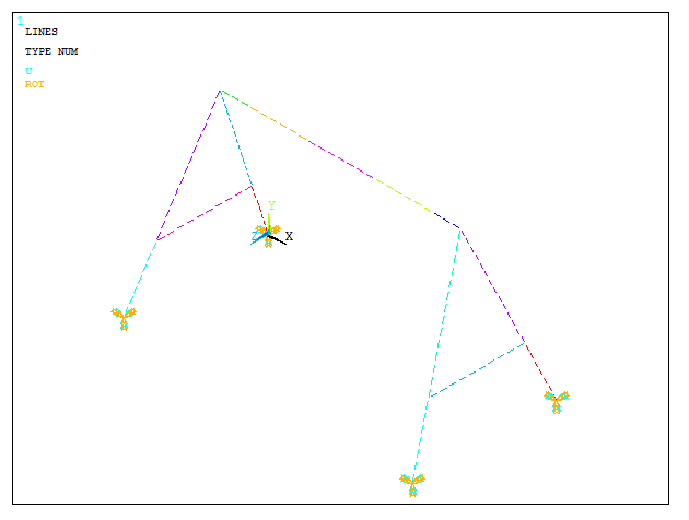
Figure 16. Boundary conditions for the structure.
Now, apply the loads. For the first loading condition, apply two forces of 500 N acting vertically on keypoints 6 and 7.
Main Menu > Solution > Define Loads > Apply > Structural > Force/Moment > On Keypoints
As indicated in Figure 17, apply -500 N in FY direction.
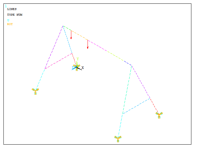
Figure 17. First loading condition.
Save the first loading condition:
Main Menu > Solution > Load Step Options > Write LS File
And define LSNUM = 1 (Figure 18).
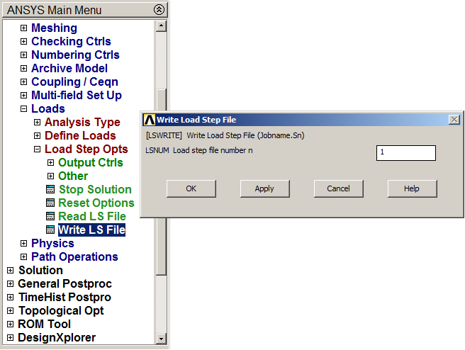
Figure 18. Saving the first loading condition.
Now, delete the forces to define the second loading condition:
Main Menu > Solution > Define Loads > Delete > Structural > Force/Moment > On Keypoints
Click "Pick All" to delete the forces and activate the numbering of keypoints:
Utility Menu > PlotCtrls > Numbering
Now select the keypoints 8 and 9 to apply two vertical forces of 500 N. On keypoints 6 and 7 apply two forces of 625 N acting at 45º (define two components of 441.94 N in FY and FZ directions):
Main Menu > Solution > Define Loads > Apply > Structural > Force/Moment > On Keypoints
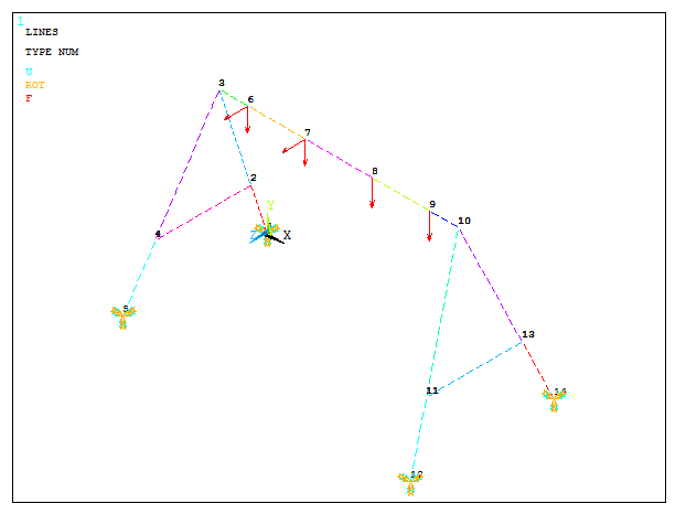
Figure 19. Second loading condition.
Again, save the second loading condition:
Main Menu > Solution > Load Step Options > Write LS File
And define LSNUM = 2.
Delete the forces and define the third loading condition:
Main Menu > Solution > Define Loads > Delete > Structural > Force/Moment > On Keypoints
Click on keypoints 8 and 9.
Now, to define the force acting horizontally in the side member, delete the mesh for this line, divide it into two lines and mesh it again.
Main Menu > Preprocessor > Meshing > Clear > Lines
Select this particular line and click "OK".
Main Menu > Preprocessor > Modeling > Operate > Booleans > Divide > Line into N Ln's
Select the line and define NDIV = 2. After that, mesh again the line:
Main Menu > Preprocessor > Meshing > Size Cntrls > ManualSize > Lines > Picked Lines
Select the two lines. The element size is 0.1 m. Finish the meshing process:
Main Menu > Preprocessor > Mesh > Lines
Finally, define the force of 450 N acting in the negative FX direction.
Main Menu > Solution > Define Loads > Apply > Structural > Force/Moment > On Keypoints
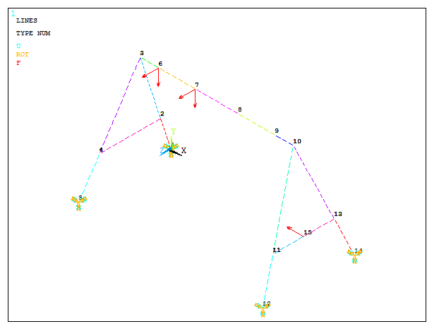
Figure 20. Third loading condition.
And save the third loading condition (LSNUM = 3):
Main Menu > Solution > Load Step Options > Write LS File
SOLUTION
Solve the problem taking into account the three loading conditions:
Main Menu > Solution > Solve > From LS Files
And define the parameters indicated in Figure 21.
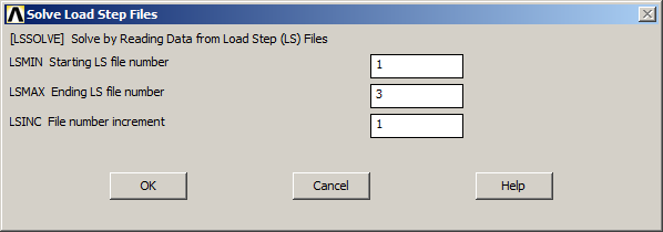
Figure 21. Solve the problem for the three loading conditions.
Click "OK" at "Solution is done!" message.
RESULTS
Evaluate the results for the first loading condition.
Main Menu > General Postproc > Read Results > First Set
Obtain the deformation of the structure:
Main Menu > General Postproc > Plot Results > Deformed Shape
And select "Def+undeformed". Figure 22 represents the deformation of the model.
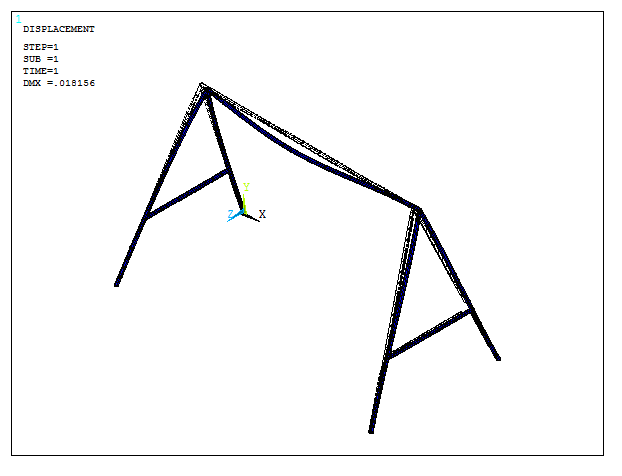
Figure 22. Deformation of the model.
The deformed model can be represented by vectors (Figure 23):
Main Menu > General Postproc > Plot Results > Vector Plot > Predefined
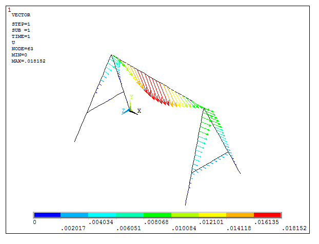
Figure 23. Deformation for the first loading condition represented by vectors.
For the second loading condition:
Main Menu > General Postproc > Read Results > Next Set
And obtain the same results for the second loading condition (Figure 24):
Main Menu > General Postproc > Plot Results > Vector Plot > Predefined
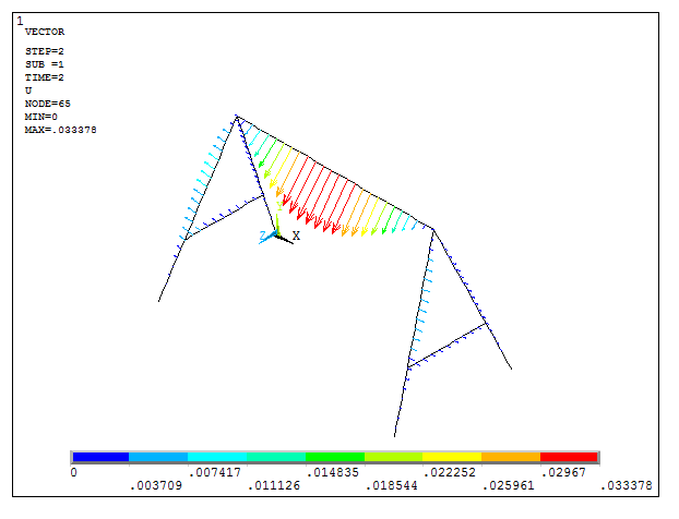
Figure 24. Deformation for the second loading condition represented by vectors.
Finally, for the third loading condition:
Main Menu > General Postproc > Read Results > Last Set
And "Replot" the results (Figure 25):
Utility Menu > Plot > Replot
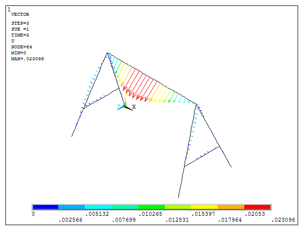
Figure 25. Deformation for the third loading condition represented by vectors.
Now, analyze the axial stresses in the structure. For the first loading condition:
Main Menu > General Postproc > Read Results > First Set
Define the labels required for the stress analysis.
For this element type, the label is "SDIR" (Axial Direct Stress):
Main Menu > General Postproc > Element Table > Define Table
For axial stresses, define SMISC 31 and 36 for i-node and j-node, respectively (ANSYS Help). And labels are "AXIAL_I" and "AXIAL_J", as indicated in Figure 26.
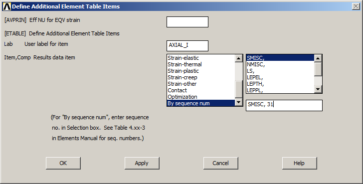
Figure 26. Labels to represent axial stresses.
Now, plot the results:
Main Menu > General Postproc > Plot Results > Contour Plot > Line Elem Res
And select "AXIAL_I" and "AXIAL_J".
The results are represented in Figure 27.
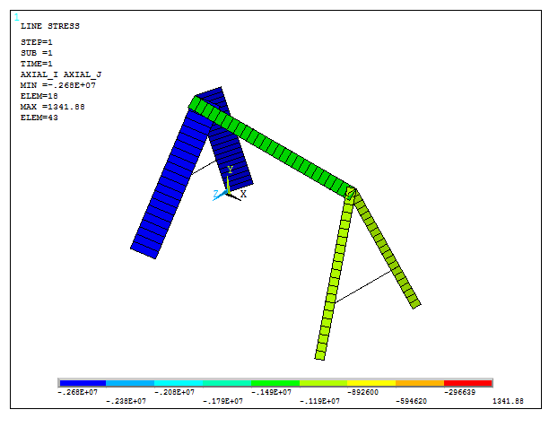
Figure 27. Axial stresses for the first loading condition.
For the second loading condition:
Main Menu > General Postproc > Read Results > Next Set
Now, update the element table:
Main Menu > General Postproc > Element Table > Define Table > Update
And plot the stress distribution (Figure 28):
Main Menu > General Postproc > Plot Results > Contour Plot > Line Elem Res
Select again "AXIAL_I" and "AXIAL_J".
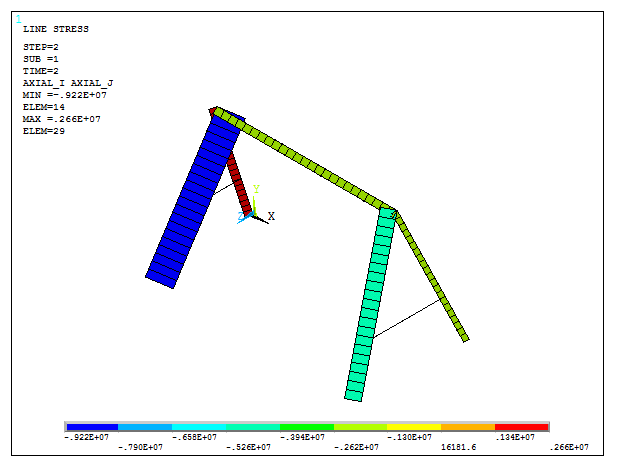
Figure 28. Axial stresses for the second loading condition.
In the same way, obtain the axial stresses for the third loading condition (Figure 29):
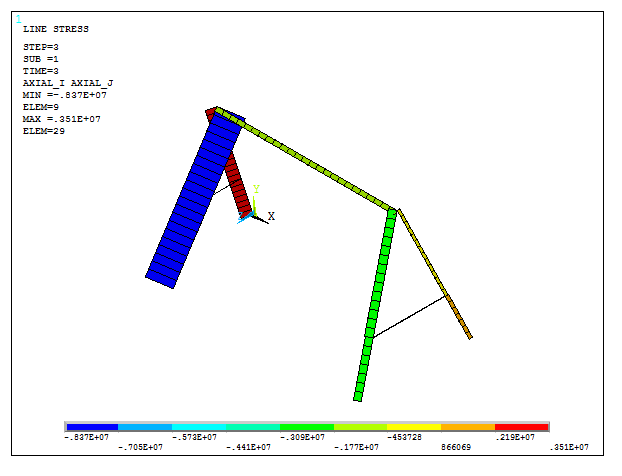
Figure 29. Axial stresses for the third loading condition.