
PROBLEM
Figure 1 represents a circular post constructed with two different bars. Bar 1 is of aluminium and bar 2 is of steel. The post is fixed at both ends.
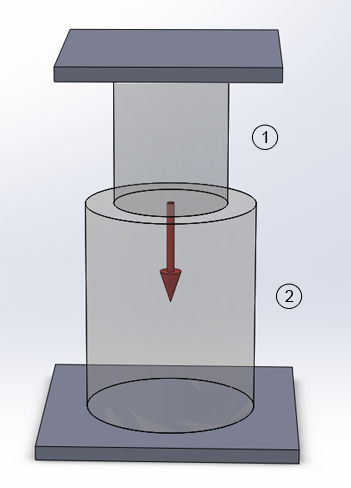
Figure 1. Circular post.
Tables 1 and 2 show the mechanical properties of the materials and the geometric characteristics, respectively.
Table 1. Material properties.
| Aluminium | Steel | ||
| Ealuminium | 69 GPa | Esteel | 210 GPa |
| Sy aluminium | 275 MPa | Sy steel | 275 MPa |
| νaluminium | 0.33 | νsteel | 0.3 |
Table 2. Geometric characteristics.
| Geometric characteristics | ||
| Element | 1 | 2 |
| Material | Aluminium | Steel |
| Area | 200 cm2 | 250 cm2 |
| Length | 100 cm | 150 cm |
The post supports a load of 1000 kN. Calculate:
GEOMETRY OF THE MODEL
First of all, a name is defined for the problem, that is "Circular post" (Figure 2):
Utility Menu > File > Change Title
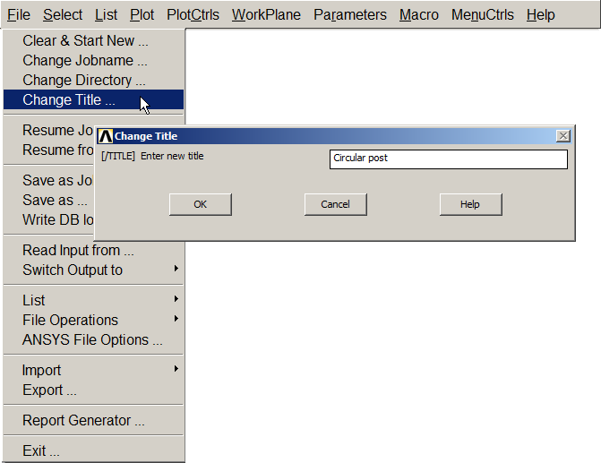
Figure 2. Name for the problem.
Next, it is defined the type of analysis for this particular problem, that is structural (Figure 3):
Main Menu > Preferences
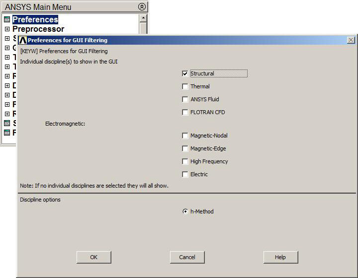
Figure 3. Structural analysis.
Now, it is very important to decide which element type is the best for each particular problem. That depends on many aspects, such as the geometry of the model and the results that are intended to obtain.
For this particular problem, it is used the LINK element, that is suitable for bars supporting axial loads (Figure 4):
Main Menu > Preprocessor > Element Type > Add/Edit/Delete > Add > LINK
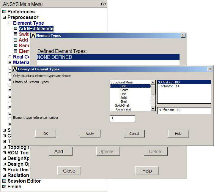
Figure 4. Element type LINK.
It is necessary to define the cross section for the bars. This will be done by means of the "Real Constants" option (Figure 5):
Main Menu > Preprocessor > Real Constants > Add/Edit/Delete
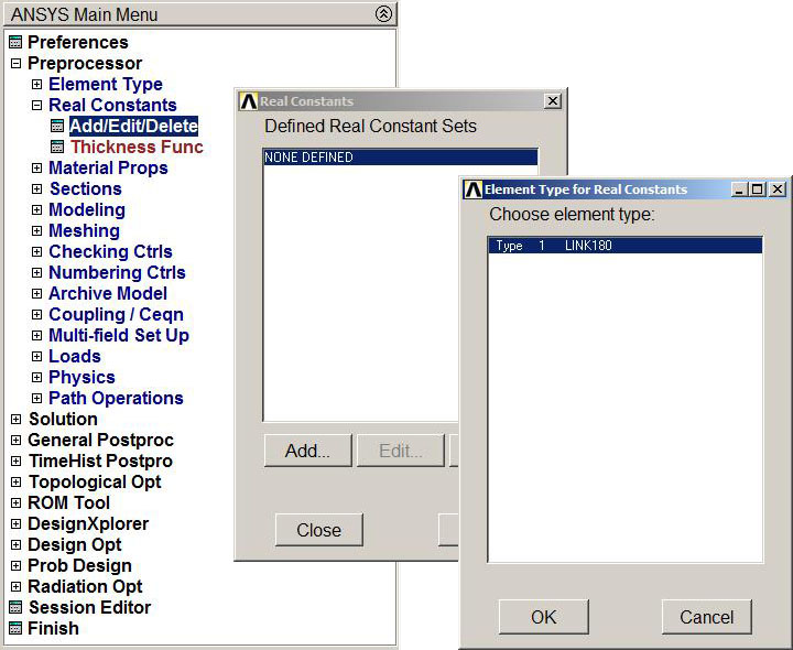
Figure 5."Real Constants" for the LINK element.
Figures 6 and 7 show the definition of the cross sectional areas for the upper bar and the lower bar, respectively.
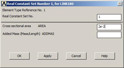
Figure 6. Cross section for the upper bar.
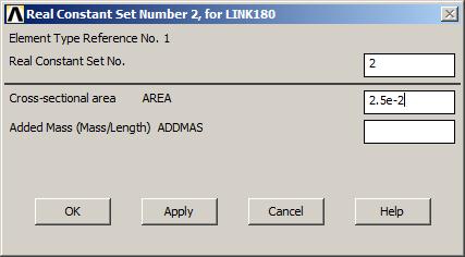
Figure 7. Cross section for the lower bar.
After the definition of the areas, Figure 8 is the window that appears when the real constants have been defined.
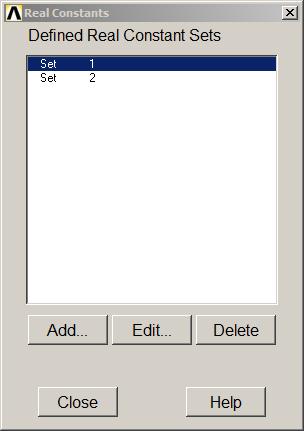
Figure 8. Defined Real Constants Sets.
From the data of Table 1, the modulus of elasticity (EX) and the Poisson's ratio (PRXY) are required for each material. We define the aluminium, as material 1 (Figure 9):
Main Menu > Preprocessor > Material Props > Material Models
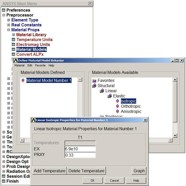
Figure 9. Aluminium properties (material 1).
In the same way, the steel properties are defined as material 2 (Figure 10):
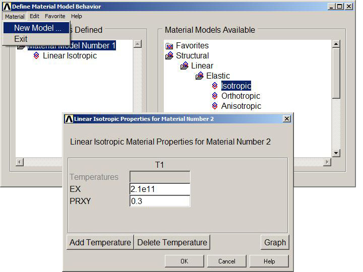
Figure 10. Steel properties (material 2).
The bars are modelled as two connected straight lines, so three nodes have to be created (Figure 11):
Main Menu > Preprocessor > Modeling > Create > Nodes > In Active CS
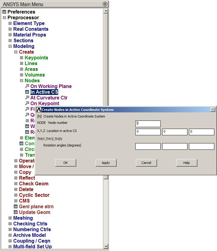
Figure 11. Creating nodes.
Table 3 shows the coordinates for the three nodes:
Table 3. Coordinates for the nodes.
| NODE | X (m) | Y (m) |
| 1 | 0 | 2.5 |
| 2 | 0 | 1.5 |
| 3 | 0 | 0 |
Figure 12 is the graphic screen with the three nodes.
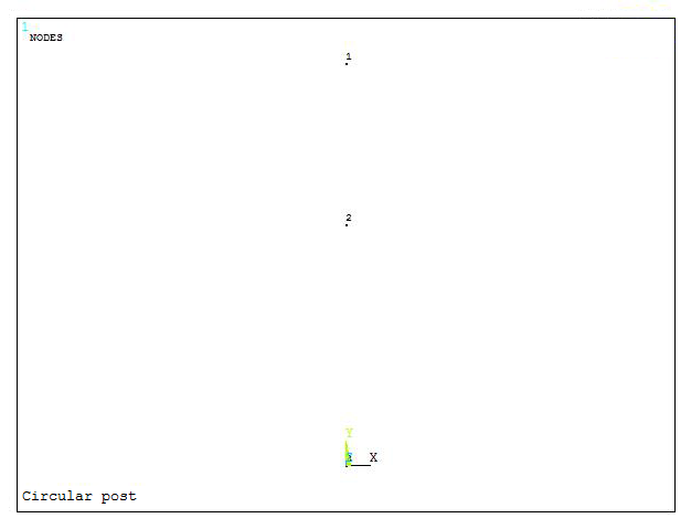
Figure 12. Graphic screen with the nodes.
In order to differentiate the two materials, it is necessary to assign attributes to each bar. First, the attributes to bar 1 (Figure 13):
Main Menu > Preprocessor > Modeling > Create > Elements > Elem Attributes
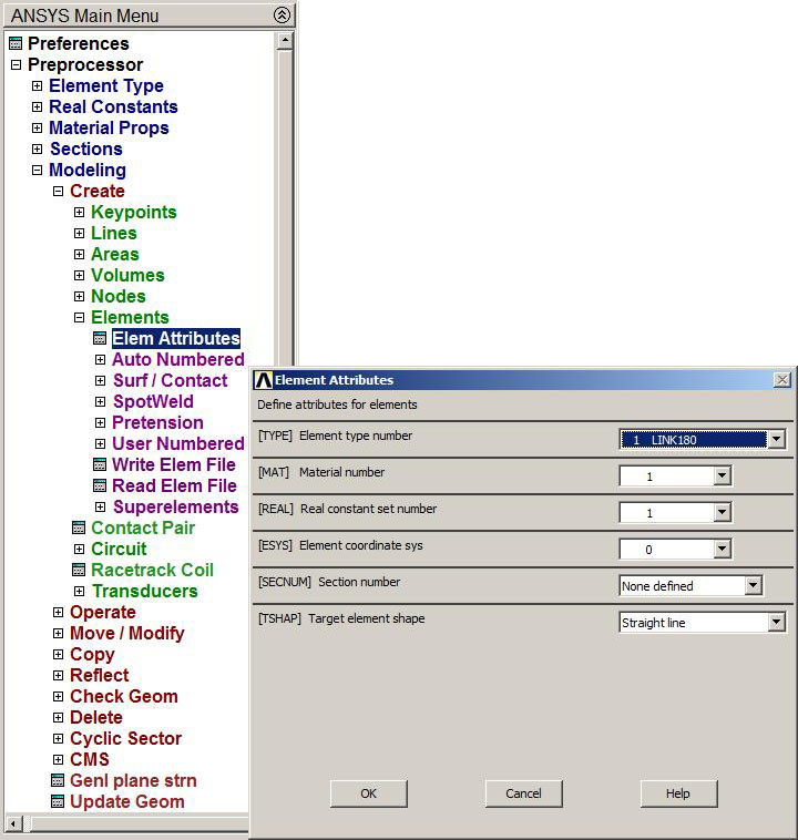
Figure 13. Element attributes for bar 1.
Now the bar 1 is created from node 1 to node 2 (Figure 14):
Main Menu > Preprocessor > Modeling > Create > Elements > Auto Numbered > Thru Nodes
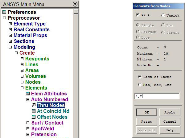
Figure 14. Creating bar 1.
The same process has to be repeated in order to assign attributes to bar 2 with the steel properties (Figure 15).
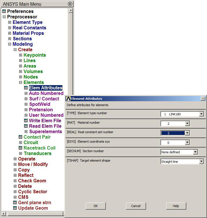
Figure 15. Element attributes for bar 2.
And now, bar 2 is created from node 2 to node 3 (Figure 16).

Figure 16. Creating bar 2.
Figure 17 shows the graphic screen with the straight lines that define the model.
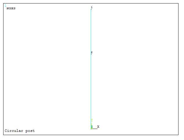
Figure 17. Defined model.
LOADS AND BOUNDARY CONDITIONS
Now that the geometry of the model has been defined, the next step is to apply the loads and the restrictions to the model (Figure 18):
Main Menu > Preprocessor > Loads > Define Loads > Apply > Structural > Displacement > On Nodes
Both ends are fixed, so they have to be constrained with "ALL DOF" option (All Degrees of Freedom).
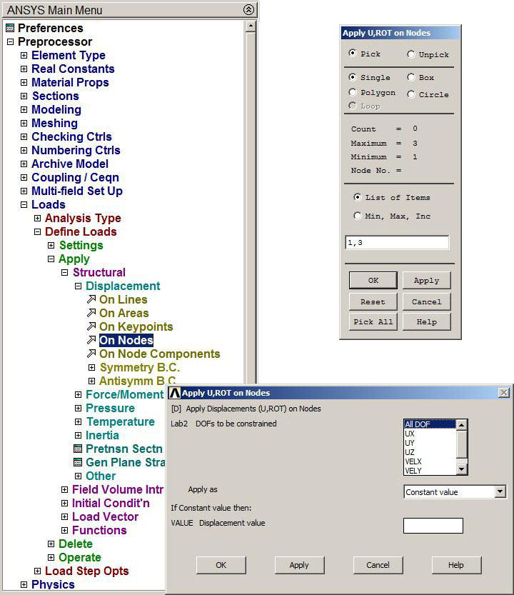
Figure 18. Fixed ends.
Figure 19 shows the graphic screen with the constrained model.
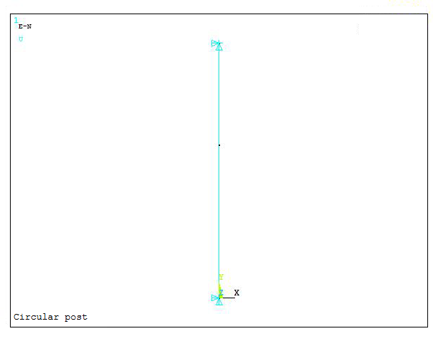
Figure 19. Constrained model.
Then, the force is applied at node 2 (Figure 20):
Main Menu > Preprocessor > Loads > Define Loads > Apply > Structural > Force/Moment > On Nodes
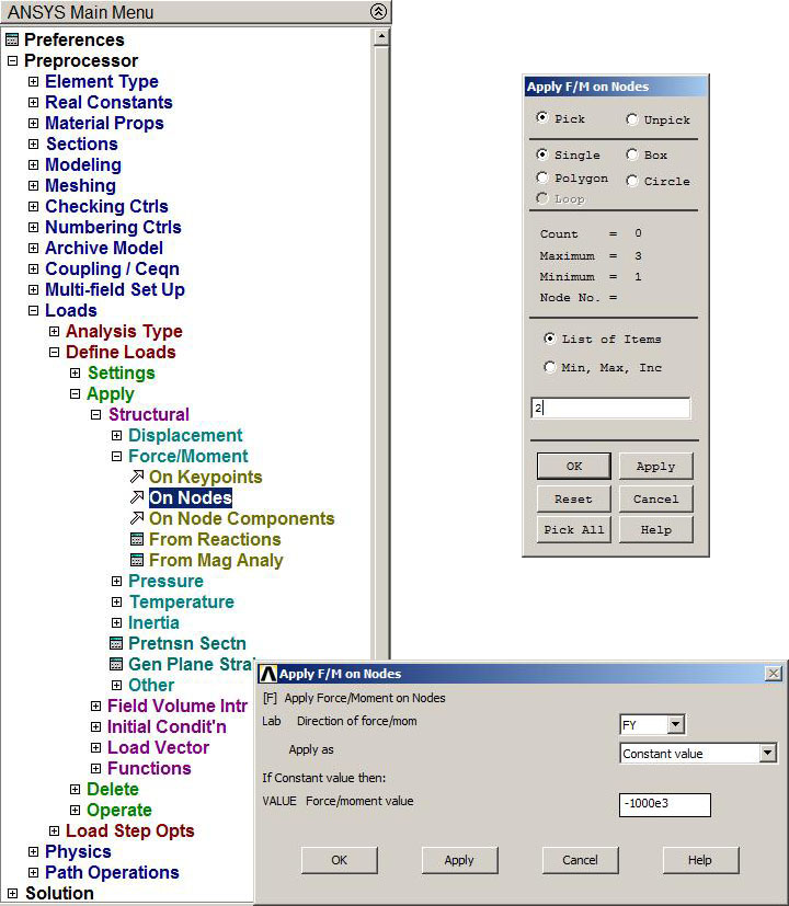
Figure 20. Applying the force.
Figure 21 shows the model with the applied force.
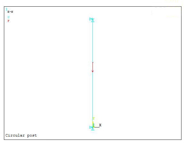
Figure 21. Applied force.
SOLUTION
When loads and boundary conditions have been defined to the model, then it has to be solved:
Main Menu > Solution > Solve > Current LS
If everything is defined in the correct way, it will appear the message "Solution is done!" (Figure 22):
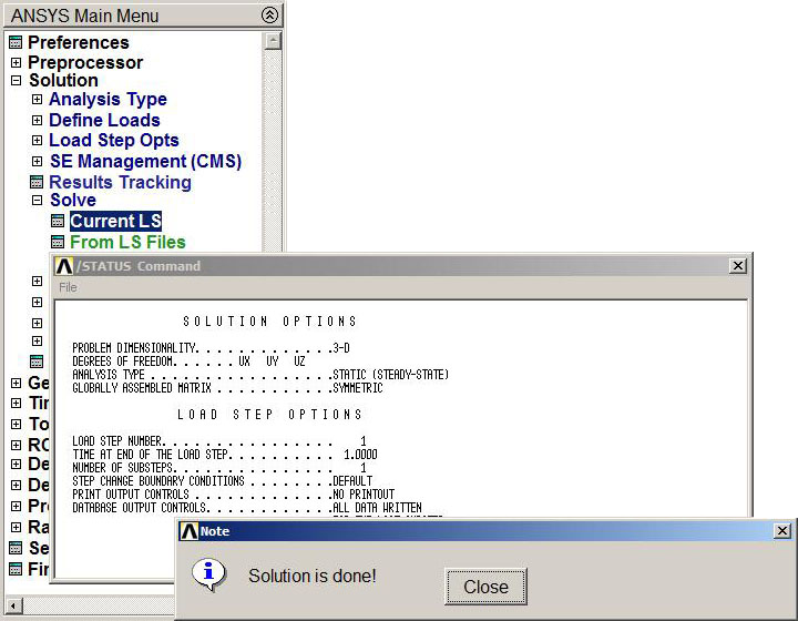
Figure 22. Solve the problem.
RESULTS
Finally, the results are analyzed. For this purpose, the "General Postprocessor" from the Main Menu is used. First of all, the deformation of the model with the option "Def + undef edge" (Figure 23):
Main Menu > General Postproc > Plot Results > Deformed Shape
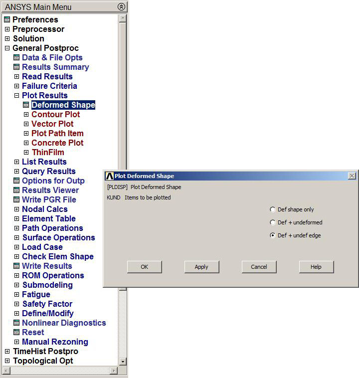
Figure 23. Deformation "Def + undef edge".
Figure 24 shows the graphic screen that represents the deformation with the maximum value (DMX), that is 0.205 mm.
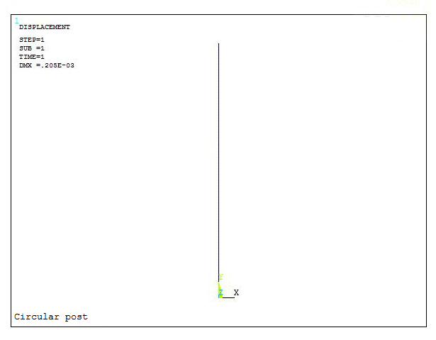
Figure 24. Maximum deformation.
The results can be seen with an option that represents the model with the real sections (Figure 25):
Utility Menu > Plot Controls > Style > Size and Shape
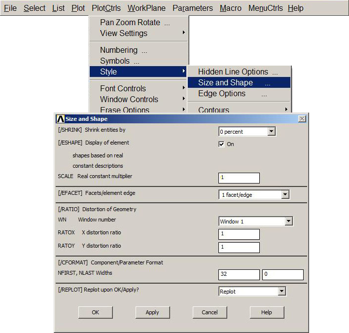
Figure 25. "Size and Shape" option.
After applying the "Size and Shape" option, the results for this particular model are represented in Figure 26.
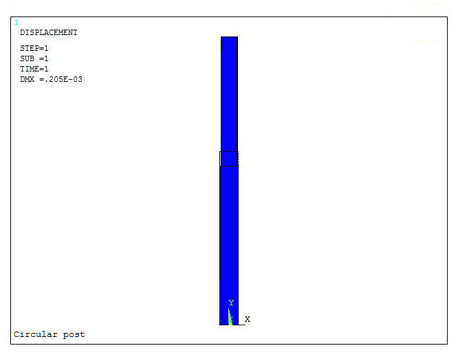
Figure 26. Scaled model.
Now, the value for the external reactions (Figure 27):
Main Menu > General Postproc > List Results > Reaction Solu
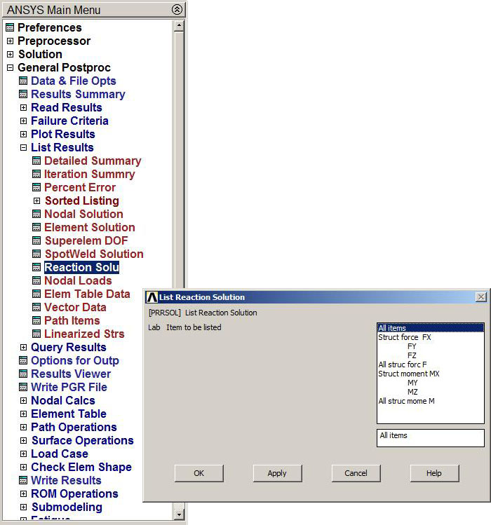
Figure 27. External reactions.
And Figure 28 shows the list for the external reactions.
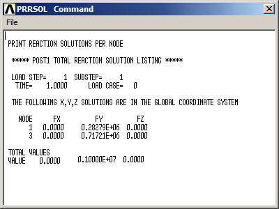
Figure 28. List of the external reactions.
Then, to obtain the value for the stresses, it is used the option "Define Table":
Main Menu > General Postproc > Element Table > Define Table
And a new label is created in order to represent the stress for the LINK element.
Figure 29 shows the window in which a label is defined in ETABLE. This label is AXIALSTR. Next, we select "By sequence num" and "LS" and type 1 (ANSYS HELP).
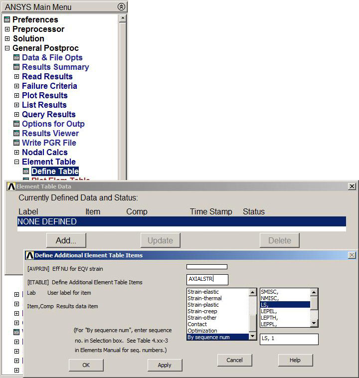
Figure 29. "Element Table".
This "Element Table Data" is showed in Figure 30.
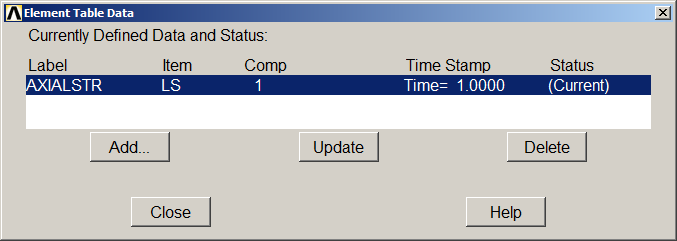
Figure 30. "Element Table Data".
Finally, to represent the distribution of stresses in the model, it is used the option "Plot Elem Table" (Figure 31):
Main Menu > General Postproc > Element Table > Plot Elem Table
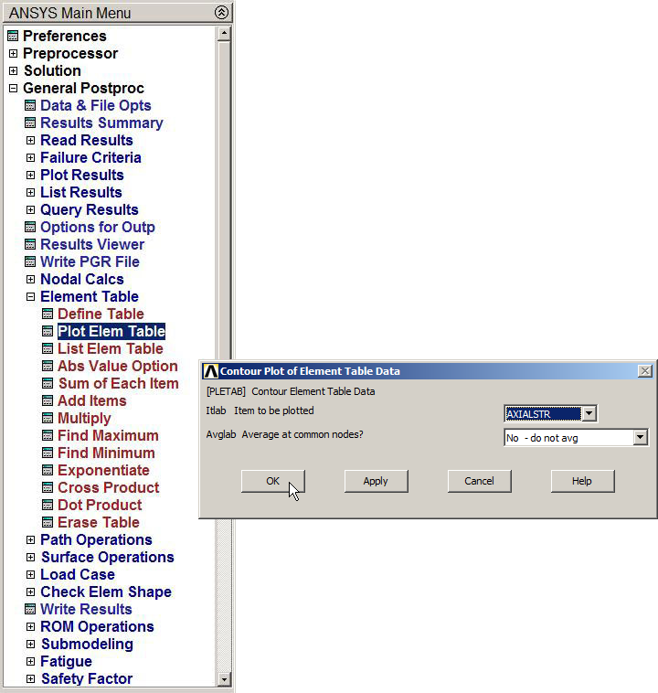
Figure 31. "Plot Element Table".
And the distribution of stresses in the circular post is showed in Figure 32.
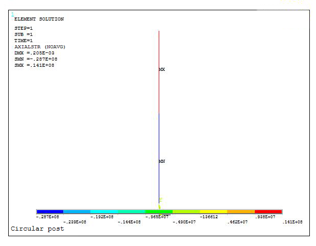
Figure 32. Stress distribution in the model.
The results indicate that the aluminium bar supports 28.7 MPa. This is the maximum value, what means that the post is safe since the elastic limit for the material is 275 MPa.