
PROBLEM
A model of a snap fit is represented in Figure 1a. The snap fit is made of polypropylene APPRYL 3120 MU 5. The mechanical properties of this material depend on the temperature (Figure 1b). Check the model for two different temperatures: 20 ºC and 80ºC. The allowable deformation has the same value as the thickness.
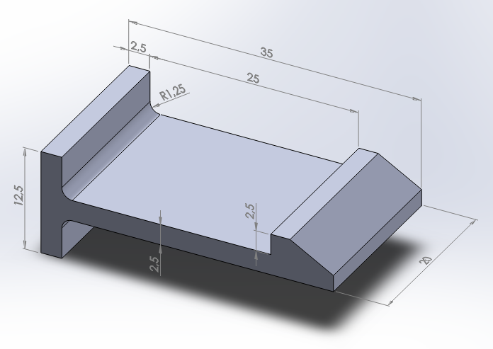
Figure 1a. Snap fit model.
Table 1 indicates the mechanical properties of the material for different temperatures.
Table 1. Material properties for different temperatures.
| POLYPROPYLENE APPRYL 3120 MU 5 (ATO) | |||||||||
| -30 ºC | 23 ºC | 60 ºC | 100 ºC | 120 ºC | |||||
| ε (%) | σ (MPa) | ε (%) | σ (MPa) | ε (%) | σ (MPa) | ε (%) | σ (MPa) | ε (%) | σ (MPa) |
| 0 | 0 | 0 | 0 | 0 | 0 | 0 | 0 | 0 | 0 |
| 0.01 | 0.372 | 0.03 | 0.4 | 0.0333 | 0.2 | 0.0334 | 0.1 | 0.0304 | 0.06 |
| 0.28 | 9.7 | 0.9 | 9.74 | 0.979 | 4.6 | 1.1 | 2.6 | 1.2 | 1.9 |
| 0.6 | 19.3 | 1.73 | 15 | 1.9 | 7.2 | 2.2 | 4.1 | 2.2 | 2.9 |
| 0.9 | 27.1 | 2.5 | 17.6 | 2.9 | 8.9 | 3.3 | 5.1 | 3.3 | 3.6 |
| 1.2 | 33.9 | 3.4 | 19.3 | 3.8 | 10.1 | 4.4 | 5.7 | 4.34 | 4.03 |
| 1.5 | 39.2 | 4.2 | 20.4 | 4.8 | 10.9 | 5.6 | 6.1 | 5.4 | 4.3 |
| 1.79 | 42.8 | 5.1 | 21.3 | 5.8 | 11.4 | 6.7 | 6.4 | 6.6 | 4.5 |
| 2 | 44.3 | 5.9 | 21.8 | 6.7 | 11.8 | 7.8 | 6.6 | 7.7 | 4.6 |
| 2.3 | 45.2 | 6.7 | 22.2 | 7.7 | 12 | 8.9 | 6.7 | 8.7 | 4.65 |
| 2.6 | 45.3 | 7.6 | 22.4 | 8.6 | 12.2 | 10 | 6.8 | 9.8 | 4.7 |
| 2.9 | 45.5 | 8.4 | 22.5 | 9.6 | 12.3 | 11.1 | 6.85 | 10.9 | 4.72 |
| Creep | Creep | Creep | Creep | Creep | |||||
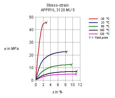
Figure 1b. Stress-strain diagram for different temperatures.
GEOMETRY OF THE MODEL
First of all, select the analysis type:
Main Menu > Preferences
Activate "Structural" option.
And change the jobname for this particular problem: "Snap fit".
Utility Menu > File > Change Jobname
For this problem, the element type is "SOLID 95", that allows to define the properties of a multilinear material. Select the element type using the ANSYS Command Prompt (Figure 2), since this element is not listed in the Main Menu.
![]()
Figure 2. "SOLID 95" element (ANSYS Command Prompt).
Now, define the mechanical properties of this polypropylene:
Main Menu > Preprocessor > Material Props > Material Models
Select the material as "Structural – Linear – Elastic – Isotropic".
Input the mechanical properties (EX and PRXY) for different temperatures ("Add Temperature"), as indicated in Figure 3.
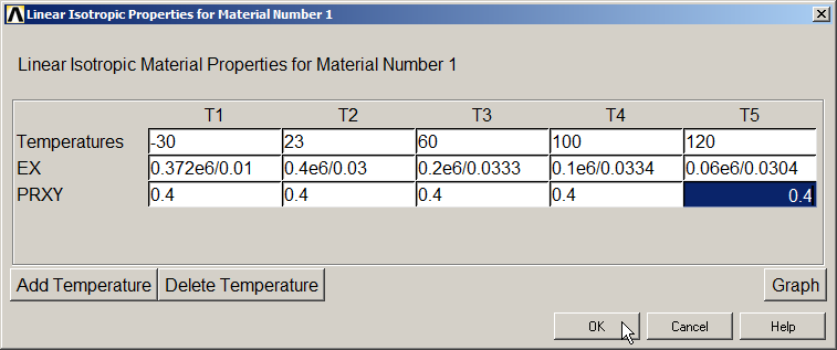
Figure 3. Defining the mechanical properties for different temperatures.
After that, from "Material Models", select "Structural – Nonlinear – Elastic – Multilinear Elastic". Figure 4 shows the input data for this material.
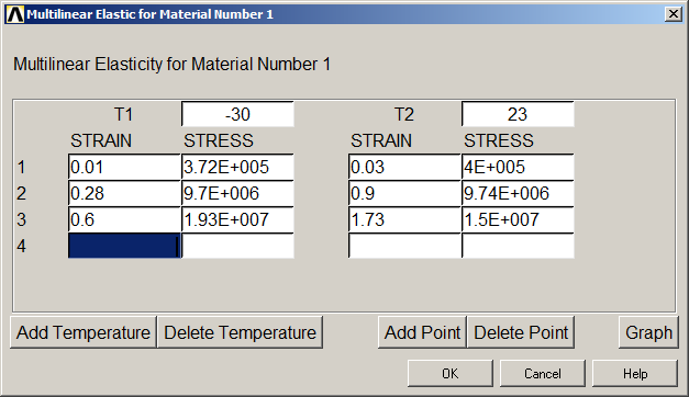
Figure 4 . Multilinear material properties.
Save the mechanical properties of the material:
Main Menu > Preprocessor > Material Props > Write to File
It is saved as "pp.SI_MPL", as indicated in Figure 5.
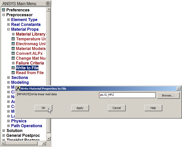
Figure 5. Save the material properties.
Figure 6 indicates the option "Read from File" for the saved material.
Main Menu > Preprocessor > Material Props > Read from File
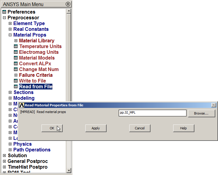
Figure 6. "Read from file" option.
Figure 7 displays the data of the material. Click on "Graph".
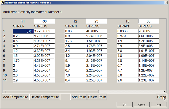
Figure 7. "Graph" option for the material data.
Stress-strain diagrams for each temperature are displayed in Figure 8.
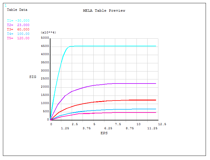
Figure 8. Stress-strain diagram for each temperature.
Now, create the model. First of all, define a grid for the working plane with the following parameters: "Snap Incr" = 0.0025 m, "Spacing" = 0.0025 m, "Minimum" = -0.036 m, "Maximum" = 0.036 m, and "Tolerance" = 0.00003 m.
Utility Menu > WorkPlane > WP Settings
The grid can be displayed with the option "Display Working Plane".
Next, create a rectangular area with the geometric characteristics indicated in Figure 9.
Main Menu > Preprocessor > Modeling > Create > Areas > Rectangle > By 2 Corners
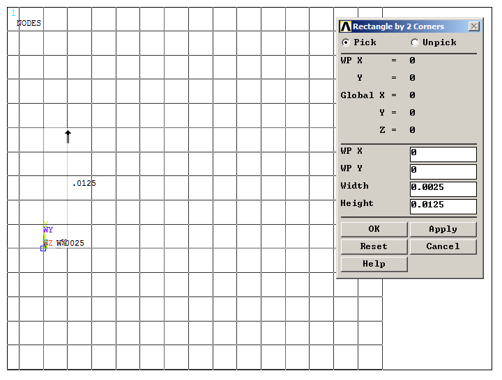
Figure 9. Creating the first rectangular area.
A second rectangular area is created as indicated in Figure 10.
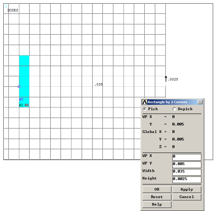
Figure 10. Creating the second rectangular area.
Finally, a third rectangular area is created as indicated in Figure 11.
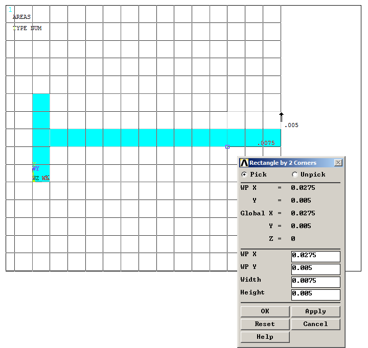
Figure 11. Creating the third rectangular area.
Apply "Add Areas" operation (Figure 12).
Main Menu > Preprocessor > Modeling > Operate > Booleans > Add >Areas
Click "Pick All".
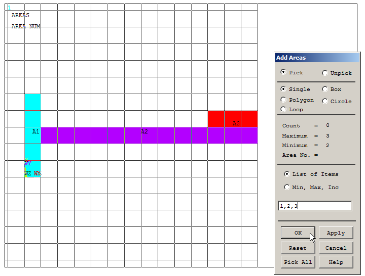
Figure 12. "Add Areas" operation.
Now, move the working plane to the keypoint 6. For this operation, number the keypoints from "Utility Menu – PlotCtrls – Numbering". Then:
Utility Menu > WorkPlane > Offset WP to > Keypoints
And select keypoint 6, as indicated in Figure 13.
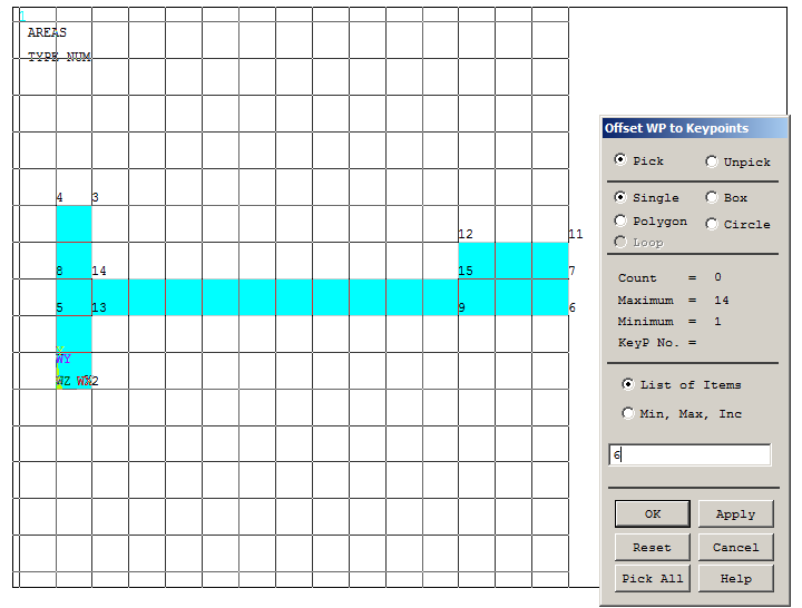
Figure 13. "Offset WP to Keypoints" to move the working plane.
Input the parameters indicated in Figure 14:
Utility Menu > WorkPlane > Offset WP by Increments
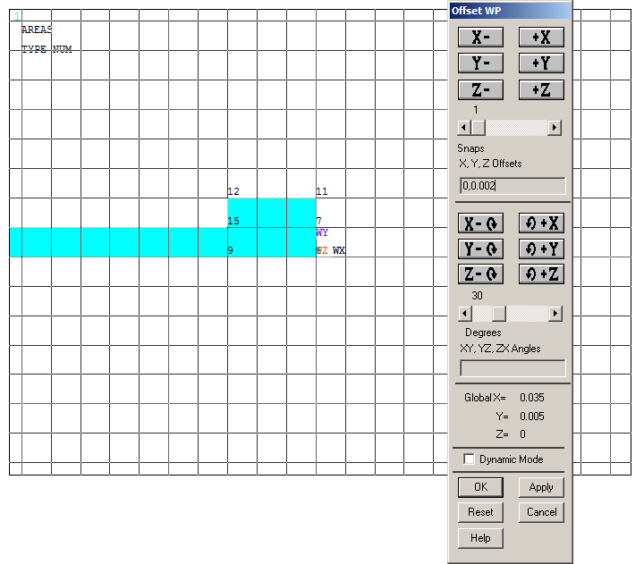
Figure 14. "Offset WP by Increments".
Now, rotate the working plane 30º in the Z axis direction, as indicated in Figure 15.
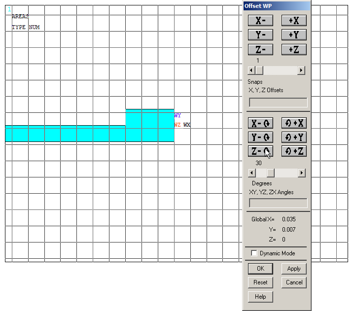
Figure 15. Rotate the working plane from "Offset WP".
After that, rotate 90º the working plane as indicated in Figure 16, from "Utility Menu – WorkPlane – Offset WP by Increments".
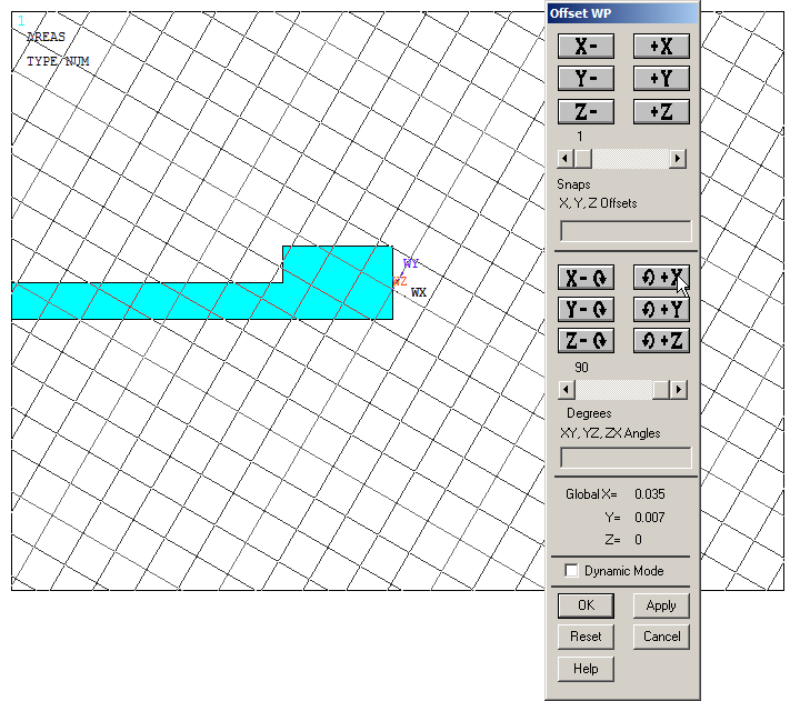
Figure 16. Rotate the working plane 90º.
Then, apply "Divide Area by WrkPlane" (Figure 17).
Main Menu > Preprocessor > Modeling > Operate > Booleans > Divide > Area by WrkPlane
Select the area and "OK".
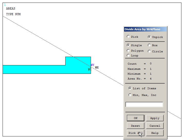
Figure 17. Divide the area by the working plane.
Now, remove the area that is not required for the model (Figure 18):
Main Menu > Preprocessor > Modeling > Delete > Area and Below
With the option "Area and Below", all the geometric entities attached to the area are deleted.
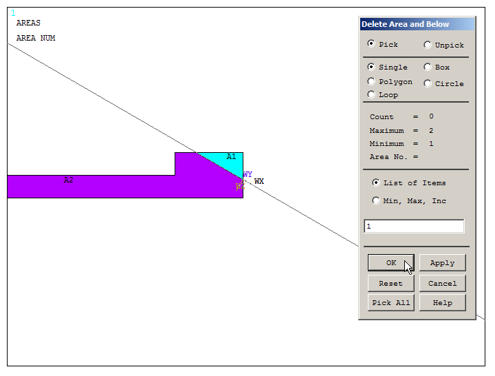
Figure 18. Delete "Area and Below".
Number the lines of the model:
Utility Menu > PlotCtrls > Numbering
Activate "Line numbers".
Then, define the radius of curvature (1.25 mm) between the lines L15 and L21 with the option "Line Fillet", as indicated in Figure 19.
Main Menu > Preprocessor > Modeling > Create > Lines > Line Fillet
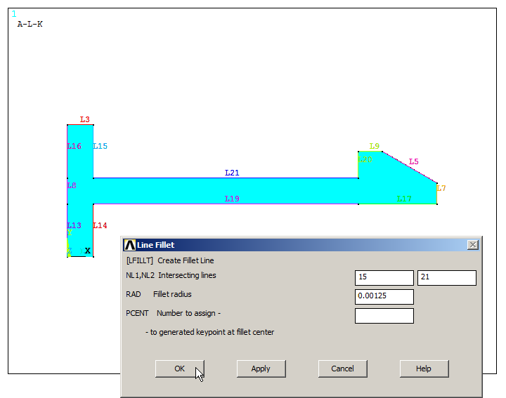
Figure 19. "Line Fillet" for the radius of curvature.
And the same radius of curvature is applied between lines L14 and L19 (Figure 20).
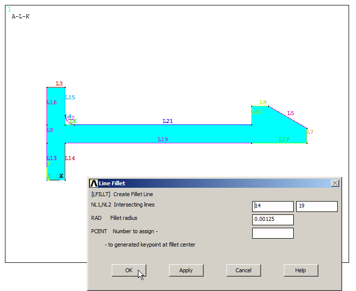
Figure 20. "Line Fillet" between lines L14 and L19.
Create the new areas defined by the lines, as indicated in Figure 21.
Main Menu > Preprocessor > Modeling > Create > Areas > Arbitrary > By Lines
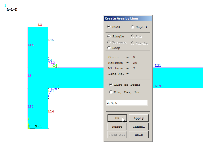
Figure 21. "Create Areas" after "Fillet" operation.
Select the lines for the new areas (Figure 22).
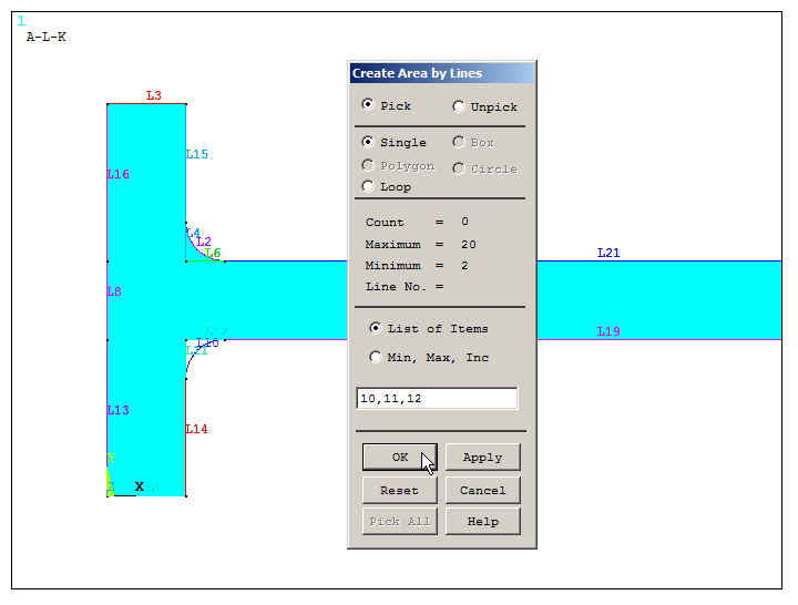
Figure 22. Creating two new areas.
Apply "Add Areas" operation, as indicated in Figure 23.
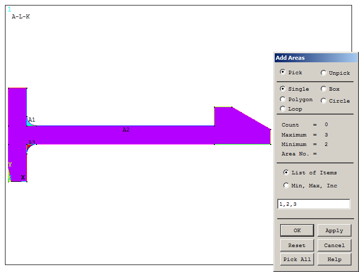
Figure 23. "Add Areas" operation.
Figure 24 displays the area for the snap fit model.
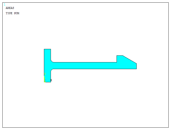
Figure 24. Created area for the model.
To check the direction of the extrusion, activate "ADIR Area direction" from "Symbols" (Figure 25).
Utility Menu > PlotCtrls > Symbols
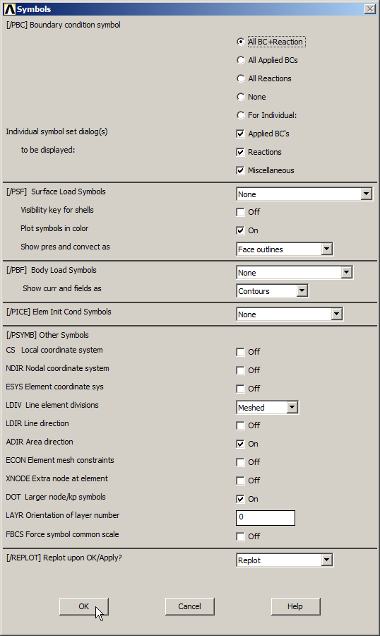
Figure 25. "ADIR" option to check the direction of the extrusion.
Figure 26 indicates the direction of the extrusion (blue arrows). It is observed the negative direction (Z axis). For this reason, the length of extrusion (DIST) is defined as negative. Its value is 20 mm.
Main Menu > Preprocessor > Modeling > Operate > Extrude > Areas > Along Normal
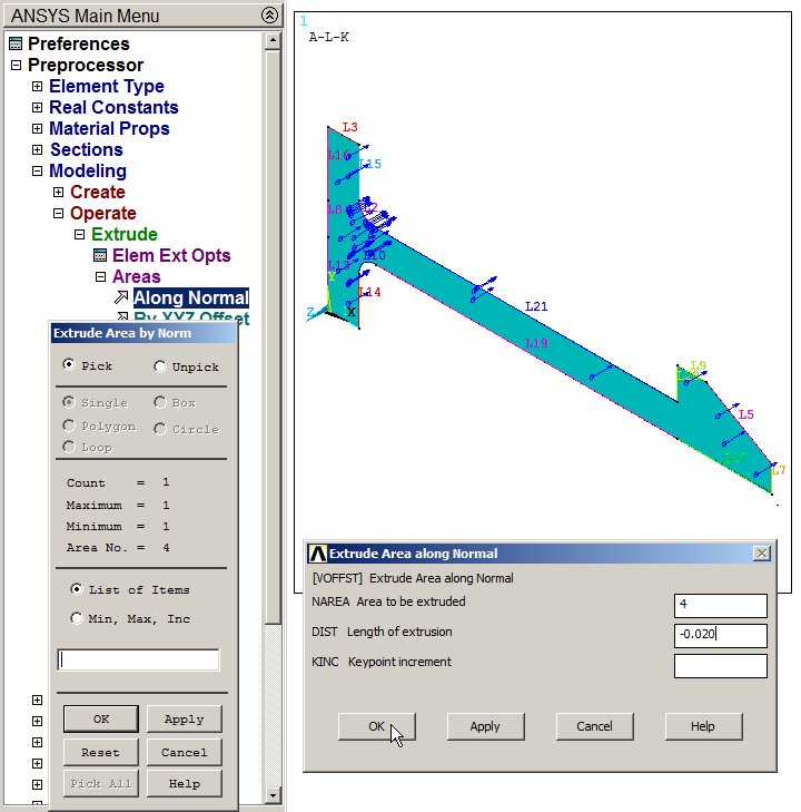
Figure 26. Direction of the extrusion for the "Extrude" operation.
Figure 27 displays the model after the "Extrude" operation. Deactivate "ADIR" option.
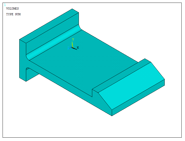
Figure 27. 3D snap fit model.
Now, mesh the model from "Mesh Tool".
Main Menu > Preprocessor > Meshing > Mesh Tool
Define the parameters indicated in Figure 28, with an element size of 0.001 m.
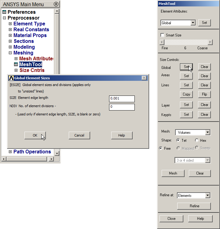
Figure 28. "Mesh Tool" option.
Figure 29 displays the meshed model after the "Sweep" operation.
Main Menu > Preprocessor > Meshing > Mesh > Volume Sweep > Sweep
Click "Pick All".
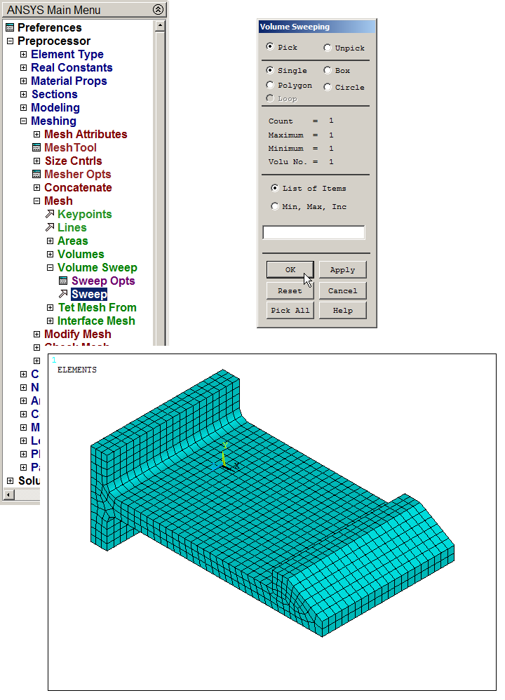
Figure 29. Meshed model after "Sweep" operation.
Number the areas, as indicated in Figure 30.
Utility Menu > PlotCtrls > Numbering
Activate "Area Numbers", then "Utility Menu – Plot – Areas".
To move and rotate the model with the mouse, activate the option "Dynamic Mode" from "Pan-Zoom-Rotate".
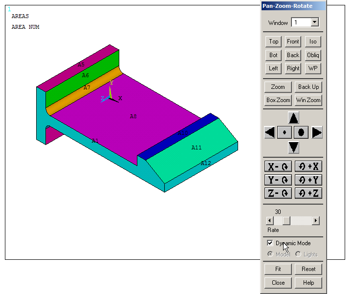
Figure 30. Plotted areas and "Dynamic Mode".
LOADS AND BOUNDARY CONDITIONS
The snap fit is fixed at the left side (areas A5 and A17). So, restrict all degrees of freedom ("All DOF") for these areas, as indicated in Figure 31.
Main Menu > Preprocessor > Loads > Define Loads > Apply > Structural > Displacement > On Areas
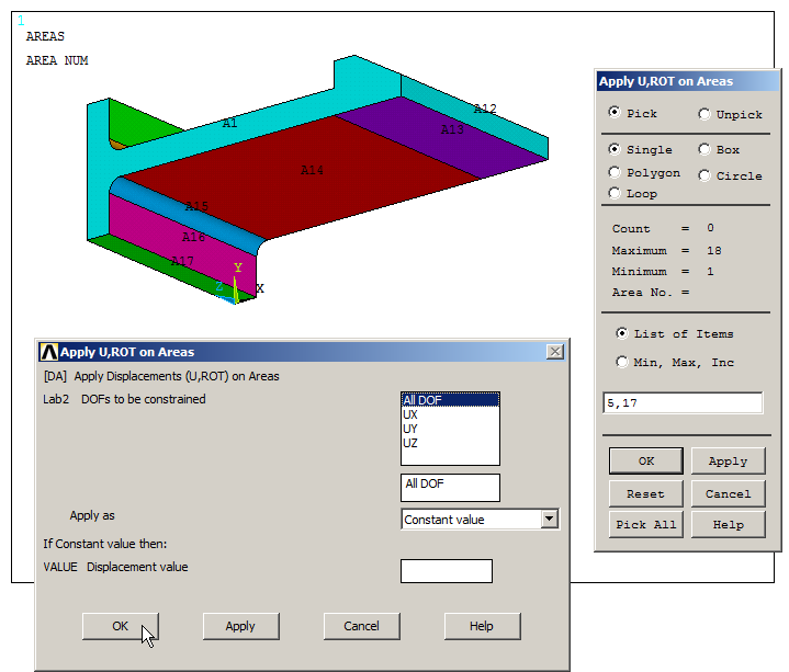
Figure 31. "All DOF" on areas A5 and A17.
Now, plot the lines of the model:
Utility Menu > Plot > Lines
And activate "Line numbers" from "Utility Menu – PlotCtrls – Numbering".
Figure 32 displays the lines of the model. Select line L40 to limit the displacement 2.5 mm in UY direction (that is the value of the thickness, as indicated in the statement of the problem).
Main Menu > Preprocessor > Loads > Define Loads > Apply > Structural > Displacement > On Lines
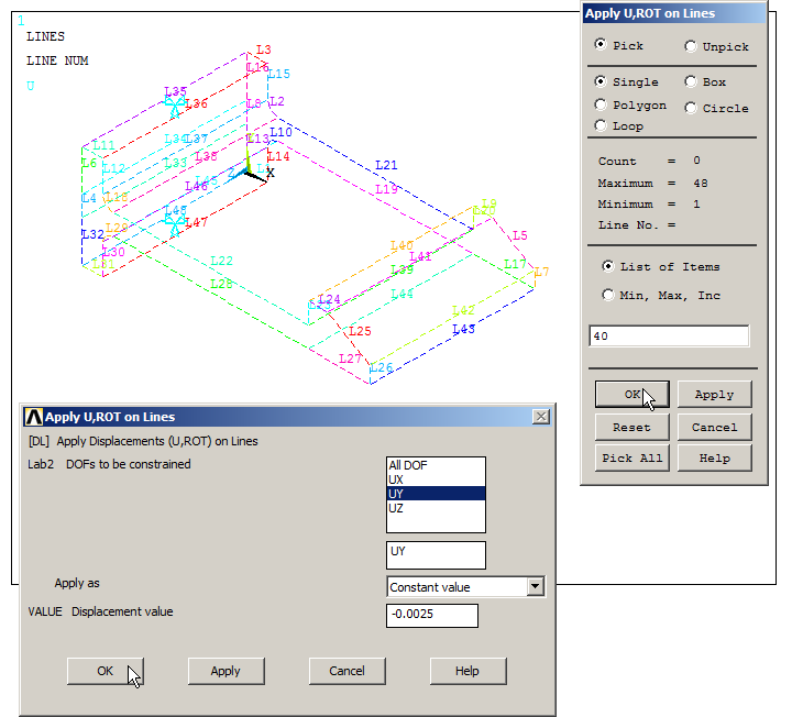
Figure 32. Restrict the displacement on line L40 (2.5 mm).
Figure 33 represents the snap fit model with the boundary conditions.
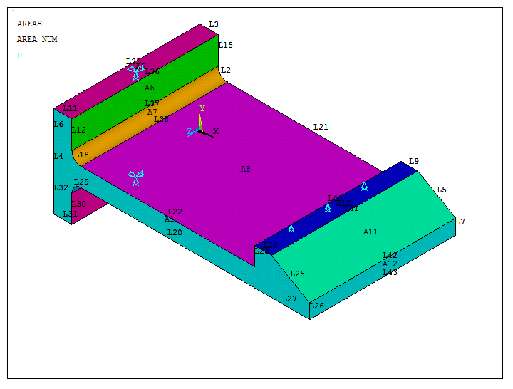
Figure 33. Snap fit with the boundary conditions.
Now, apply 20 ºC, as indicated in Figure 34.
Main Menu > Preprocessor > Loads > Define Loads > Apply > Structural > Temperature > Uniform Temp
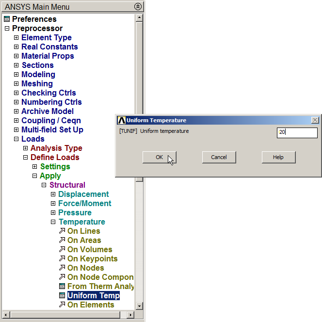
Figure 34. Apply the temperature (20 ºC).
SOLUTION
Solve the problem:
Main Menu > Solution > Solve > Current LS
"Solution is done!".
After solving the problem, Figure 35 displays the diagram "Absolute Convergence Norm" – "Cumulative Iteration Number".
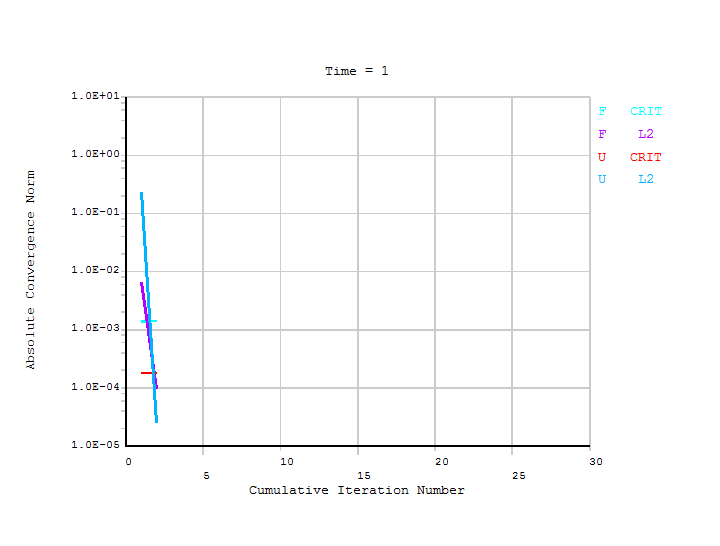
Figure 35. Diagram "Absolute Convergence Norm" – "Cumulative Iteration Number".
RESULTS
For the stress distribution in the model:
Main Menu > General Postproc > Plot Results > Contour Plot > Nodal Solu
Select "von Mises stress" (Figures 36, 37 and 38).
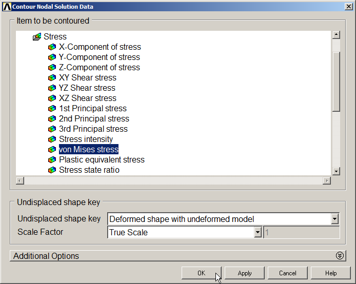
Figure 36. Select "von Mises stress" option.
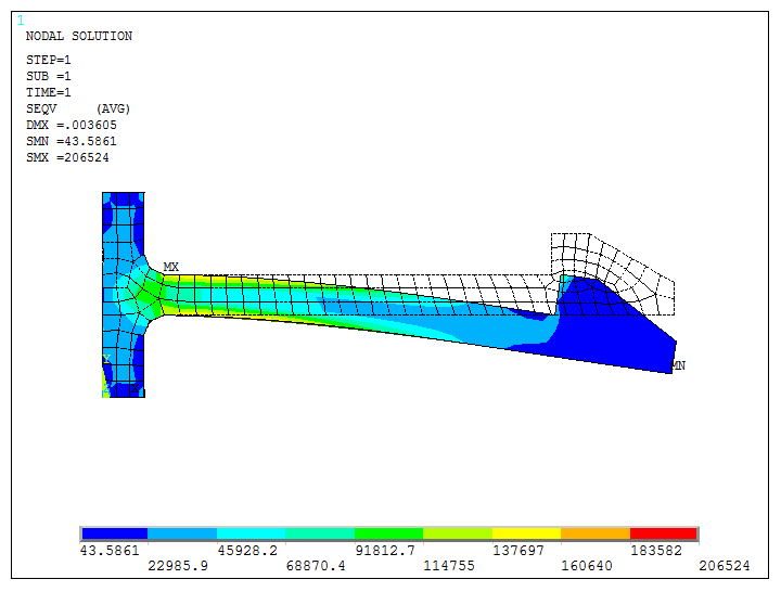
Figure 37. Stresses and deformed shape (front view).
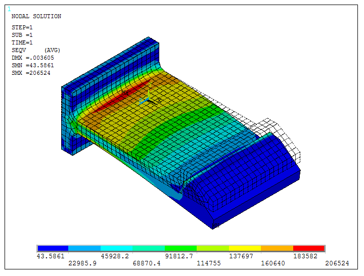
Figure 38. Stresses and deformed shape (3D view).
Now, obtain the reaction forces on line L40, where restriction has been applied.
Utility Menu > Select > Entities
Select "Lines" and "By Num/Pick". Click "OK" and select the line L40 as indicated in Figure 39.
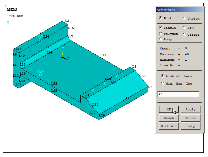
Figure 39. Select line L40.
Now, select the nodes attached to line L40 (Nodes – Attached to – Lines), as indicated in Figure 40, and click "OK".
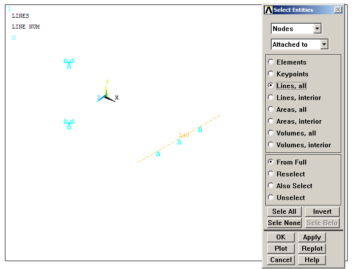
Figure 40. Selecting the nodes attached to line L40.
Reaction forces acting on the selected nodes are listed in Figure 41.
Main Menu > General Postproc > List Results > Reaction Solu
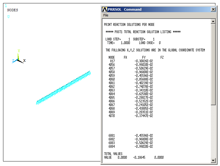
Figure 41. Reaction forces on the nodes attached to line L40.
Now, select all the geometric entities:
Utility Menu > Select > Everything
Finally, input a temperature of 80 ºC, as indicated in Figure 42.
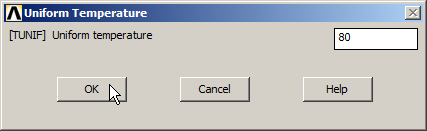
Figure 42. Applying 80 degrees Celsius.
Again, solve the problem and represent the stress distribution.
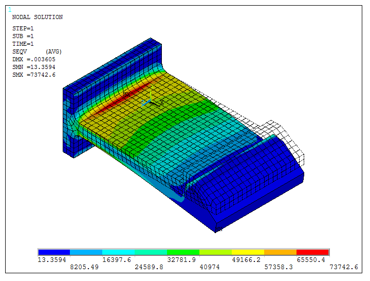
Figure 43. Stress distribution for 80 ºC.