PROBLEM
Figure 1 represents a cantilever beam with a concentrated load of 2500 N.

Figure 1. Cantilever beam.
The rectangular cross section has the dimensions 200 mm x 350 mm. Table 1 indicates the mechanical properties of the laminated steel for this beam.
Table 1. Mechanical properties.
| Laminated steel | |
| Esteel | 220 GPa |
| Sy steel | 275 MPa |
| νsteel | 0.292 |
Determine:
GEOMETRY OF THE MODEL
First of all, we define a name for the problem (Figure 2).
Utility Menu > File > Change Title
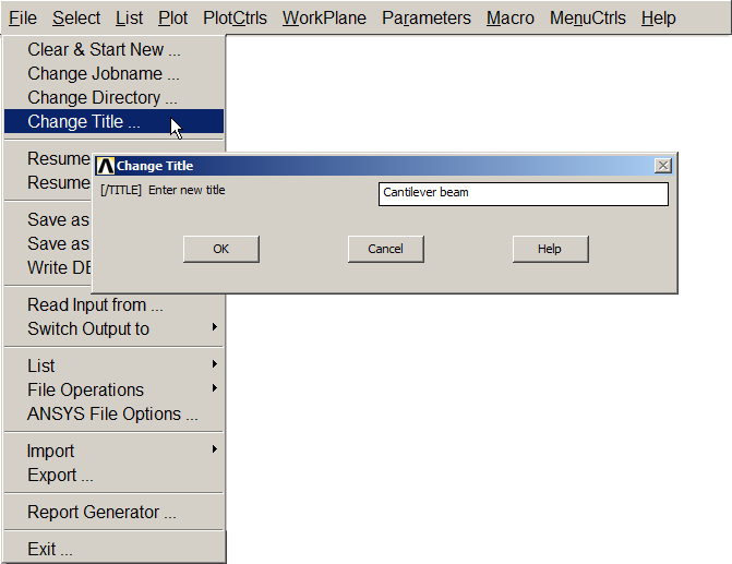
Figure 2. Change title.
Then, we select the analysis type (Figure 3):
Main Menu > Preferences
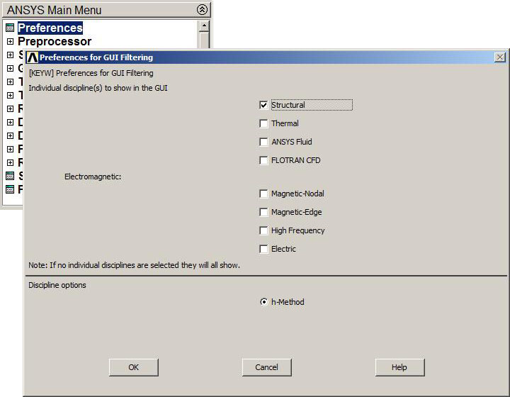
Figure 3. Structural analysis.
For this particular problem the element type is "BEAM 188" (Figure 4).
Main Menu > Preprocessor > Element Type > Add/Edit/Delete
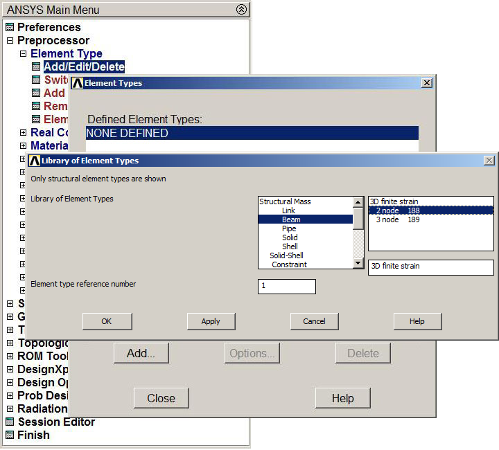
Figure 4. "BEAM 188" element.
Next, the material properties are defined (Figure 5).
Main Menu > Preprocessor > Material Props > Material Models
The material is defined as "Structural – Linear – Elastic – Isotropic".
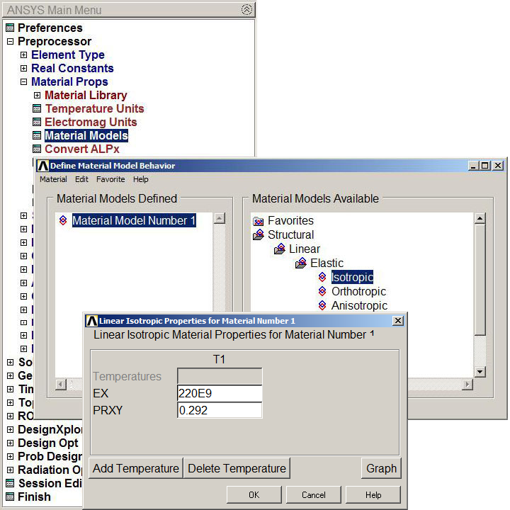
Figure 5. Mechanical properties for the laminated steel.
Figure 6 shows the "Beam Tool" display to define the dimensions of the cross section.
Main Menu > Preprocessor > Sections > Beam > Common Sections
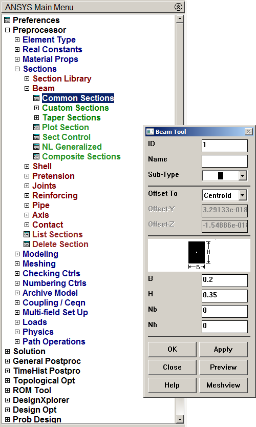
Figure 6. Dimensions for the cross section.
Now, the section can be plotted (Figure 7).
Main Menu > Preprocessor > Sections > Beam > Plot Section
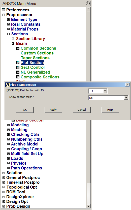
Figure 7. "Plot Section" option.
And Figure 8 is the graphic screen with the geometric properties of the section.
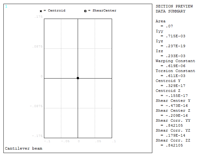
Figure 8. Geometric properties of the section.
When the section has been defined, the keypoints are created for the beam. The two keypoints are 1 (0, 0) and 2 (4, 0), as represented in Figure 9.
Main Menu > Preprocessor > Modeling > Create > Keypoints > In Active CS
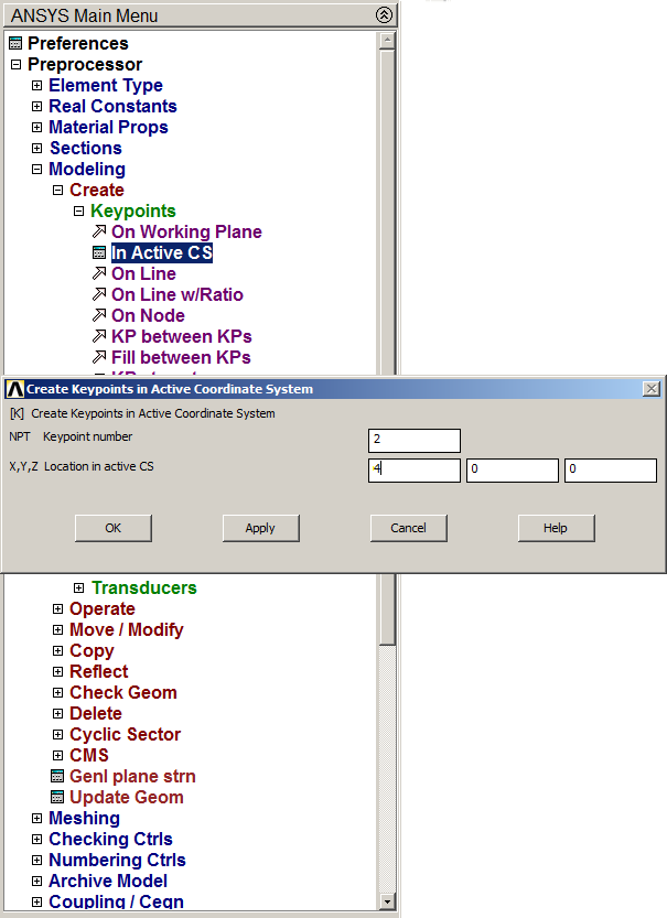
Figure 9. Create two keypoints.
The graphic screen with the two keypoints are represented in Figure 10.
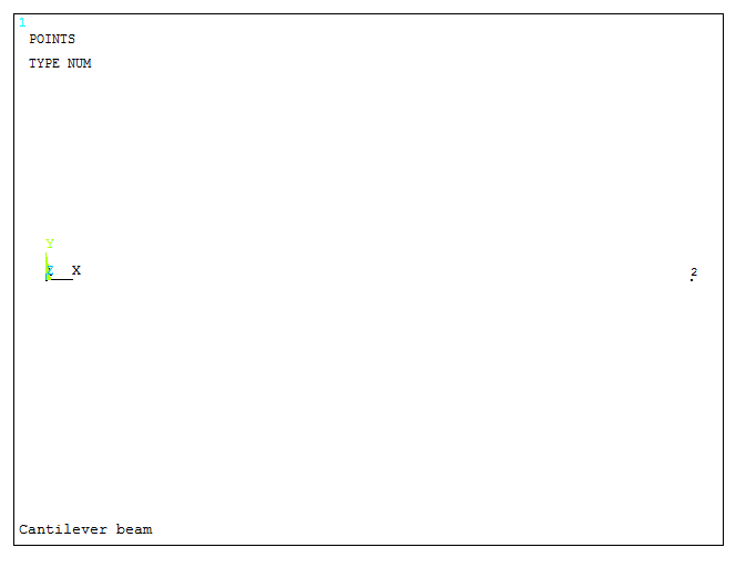
Figure 10. Graphic screen with the two keypoints.
Now, a straight line is created between the two keypoints (Figure 11).
Main Menu > Preprocessor > Modeling > Create > Lines > Straight Line
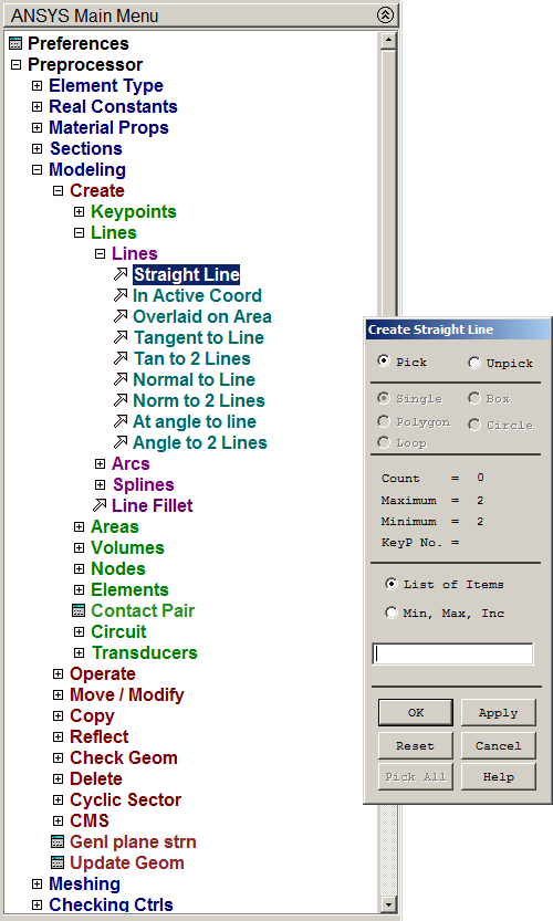
Figure 11. Create a straight line between keypoints.
Figure 12 represents the line for the cantilever beam.
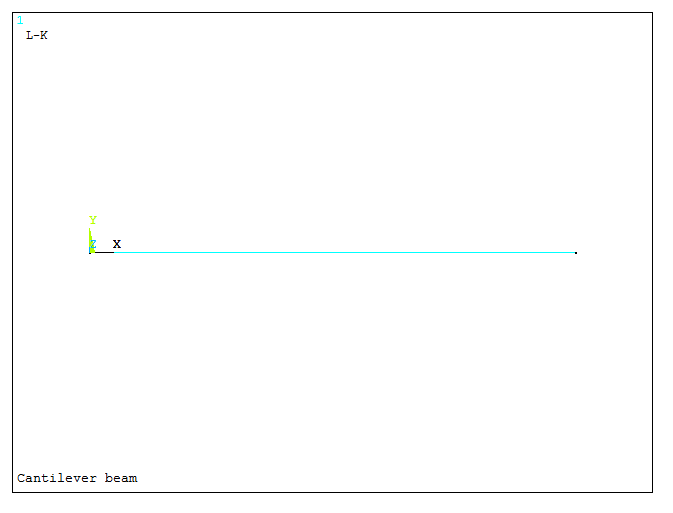
Figure 12. Line for the cantilever beam.
The model for the beam has been created. Now it has to be meshed. For this particular problem, we define a number of element divisions. As represented in Figure 13, there will be 100 element divisions.
Main Menu > Preprocessor > Meshing > Size Cntrls > Manual Size > Lines > Picked Lines
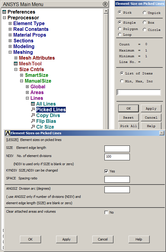
Figure 13. "Element Sizes on Lines".
To complete the meshing process (Figure 14).
Main Menu > Preprocessor > Meshing > Mesh > Lines
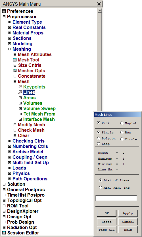
Figure 14. "Mesh Lines".
The meshed model is represented in Figure 15.
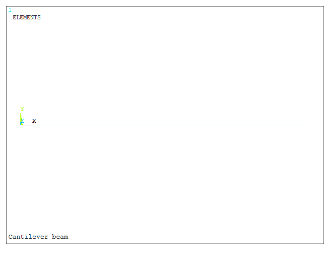
Figure 15. Meshed model.
LOADS AND BOUNDARY CONDITIONS
For the boundary conditions, the left end of the beam is fixed (Figure 16).
Main Menu > Preprocessor > Loads > Define Loads > Apply > Structural > Displacement > On Keypoints
Select the left keypoint and "All DOF" (all degrees of freedom).
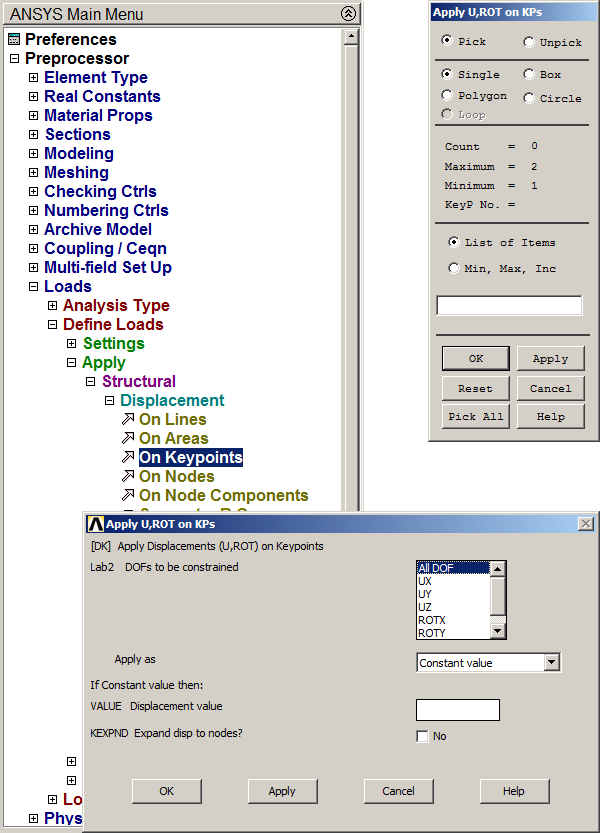
Figure 16. "All DOF" at left keypoint.
The applied restriction is represented in Figure 17.
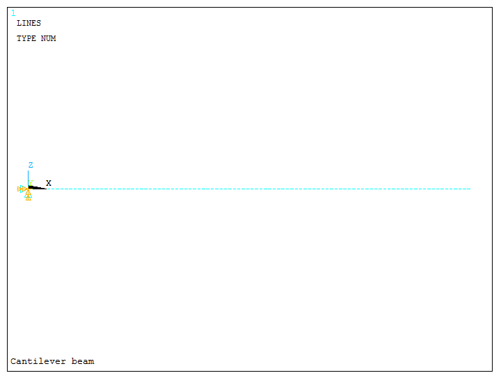
Figure 17. Fixed end.
Now, we define the load of 2500 N acting at the right end of the beam (Figure 18).
Main Menu > Preprocessor > Loads > Define Loads > Apply > Structural > Force/Moment > On Keypoints
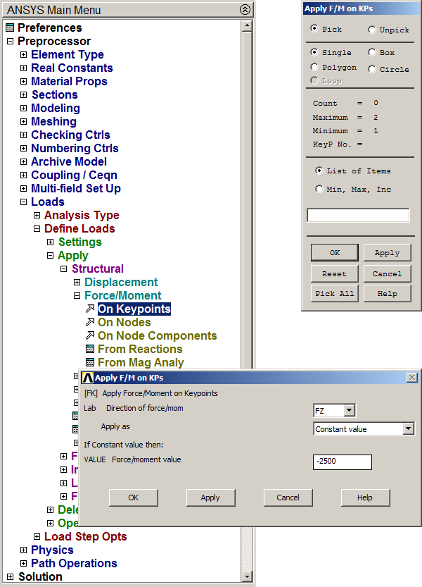
Figure 18. Applying the load.
Figure 19 represents the graphic screen with the load acting at one end of the beam.
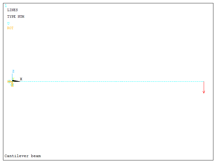
Figure 19. Beam with load at one end.
SOLUTION
When the geometric model is completed, we can solve the problem (Figure 20).
Main Menu > Solution > Solve > Current LS
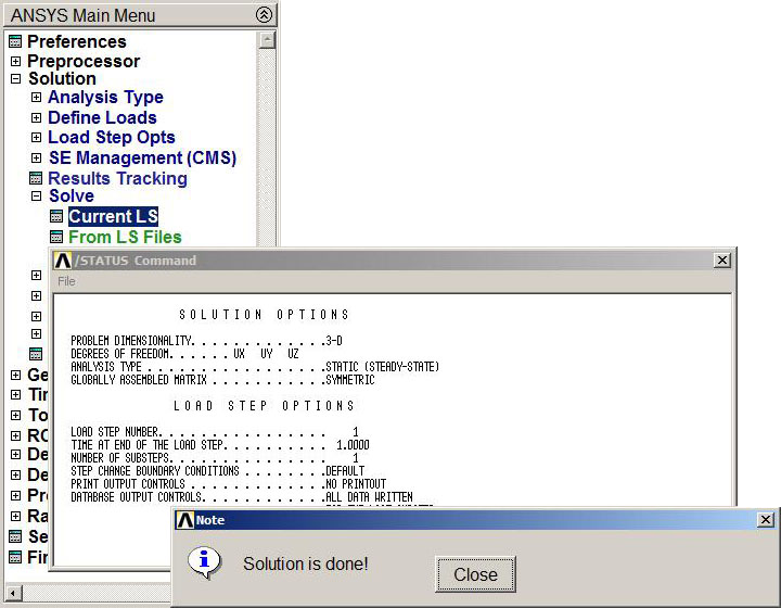
Figure 20. Solve the problem.
RESULTS
Finally, results can be analyzed. First, we evaluate the external reactions at fixed end (Figure 21).
Main Menu > General Postproc > List Results > Reaction Solu
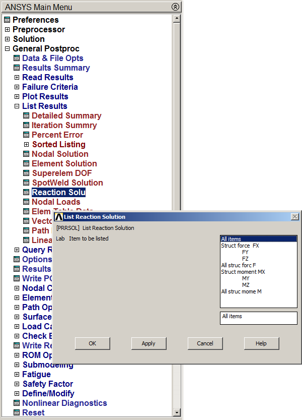
Figure 21. Obtaining external reactions.
Figure 22 shows the values for the external reactions.
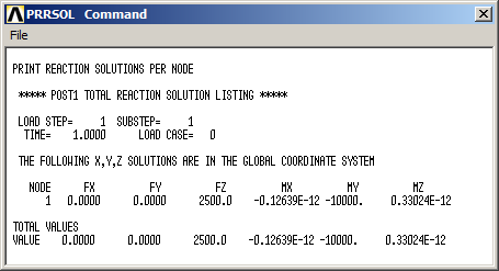
Figure 22. External reactions.
After that, deformations are analyzed (Figure 23):
Main Menu > General Postproc > Plot Results > Deformed Shape
Select "Def+undef edge".
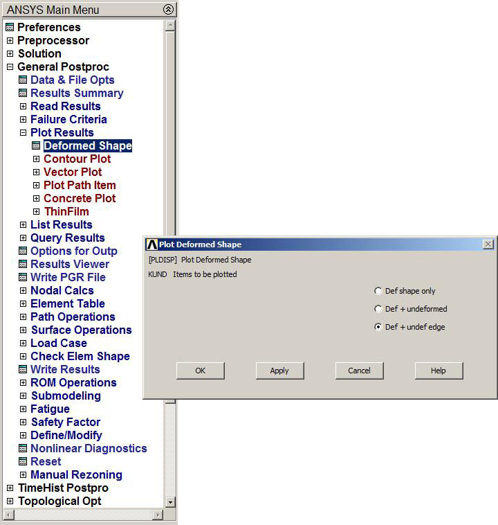
Figure 23. "Def+undef edge" option.
Figure 24 represents the graphic screen with the deflection of the beam.
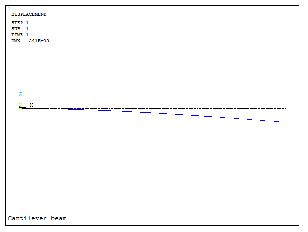
Figure 24. Deflection of the beam.
Now, diagrams for bending moments and shear forces have to be evaluated. An "Element Table" is created (Figure 25).
Main Menu > General Postproc > Element Table > Define Table
To evaluate the shear force diagram, some labels have to be created. For this particular problem "SHEARi" and SHEARj" are the labels for shear forces. Select "By sequence num" and "SMISC, 5" for i node and "SMISC, 18" for j node (ANSYS help for BEAM188).
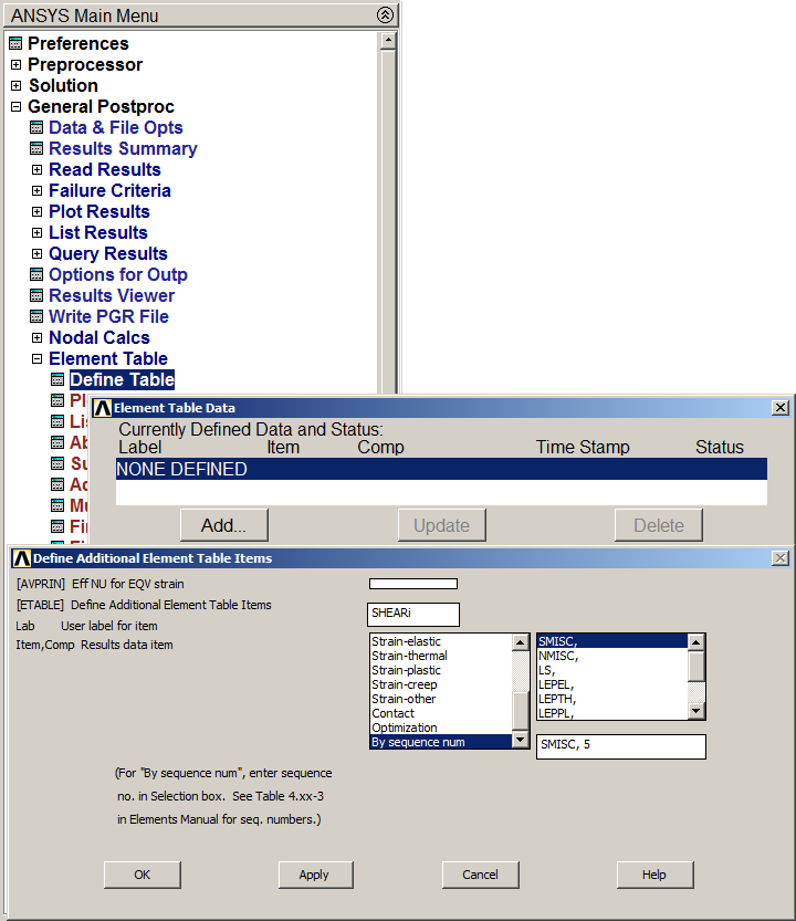
Figure 25. Element Table Data.
In the same way, "MOMi" and "MOMj" are the labels for the bending moment diagram, with the options "SMISC, 2" and "SMISC, 15", respectively (Figure 26).
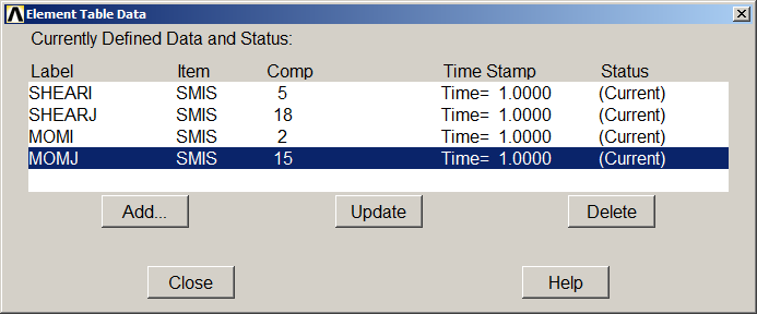
Figure 26. Labels for shear forces and bending moments.
These results can be listed (Figure 27).
Main Menu > General Postproc > Element Table > List Elem Table
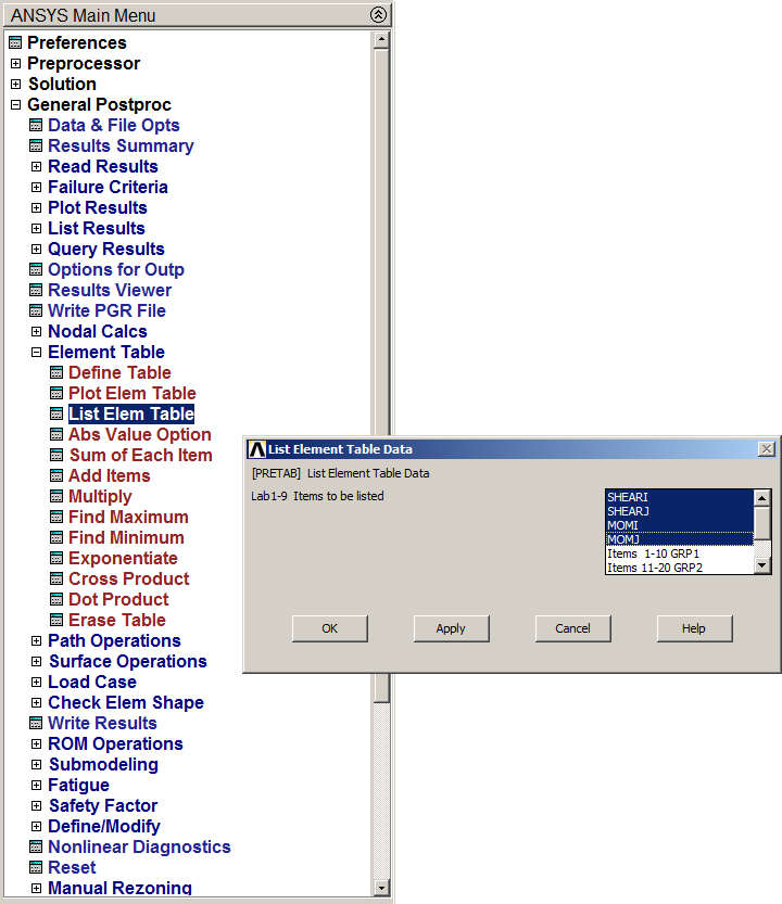
Figure 27. List Element Table Data.
The listed results are in Figure 28.
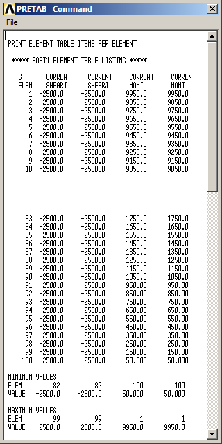
Figure 28. Listed results for shear forces and bending moments.
To represent the shear force diagram:
Main Menu > General Postproc > Plot Results > Contour Plot > Line Elem Res
And select "SHEARi" and "SHEARj" in "LabI" and "LabJ", respectively (Figure 29).
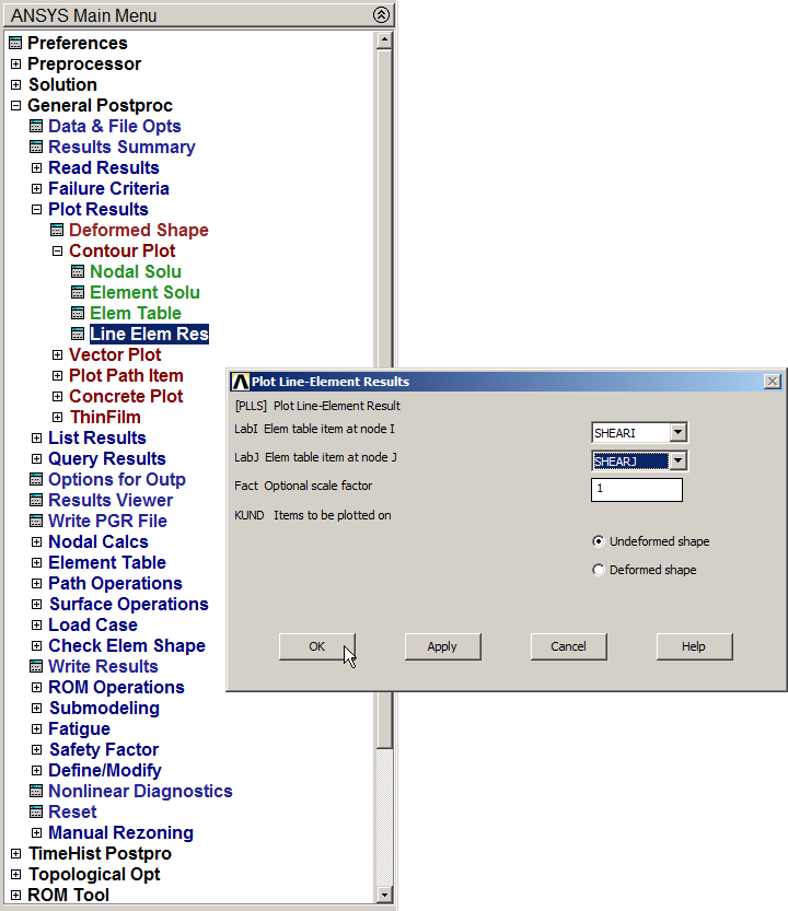
Figure 29. Plot shear forces.
Shear forces diagram is represented in Figure 30.
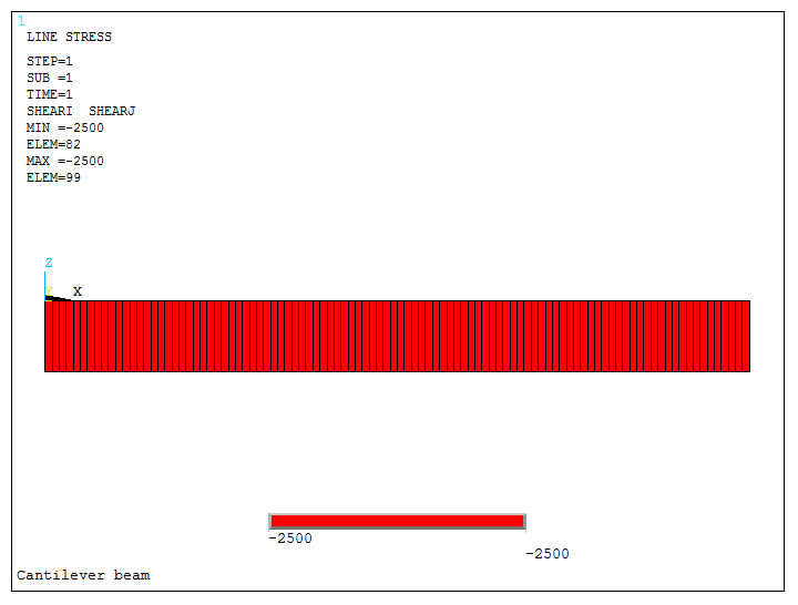
Figure 30. Shear force diagram.
Finally, to represent the bending moment diagram, select "MOMi" and "MOMj" in "LabI" and "LabJ", respectively (Figure 31).
Main Menu > General Postproc > Plot Results > Contour Plot > Line Elem Res
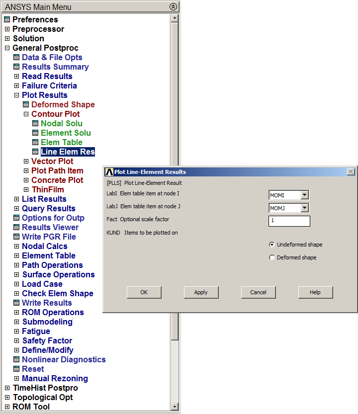
Figure 31. Plot bending moments.
Bending moments diagram is represented in Figure 32.
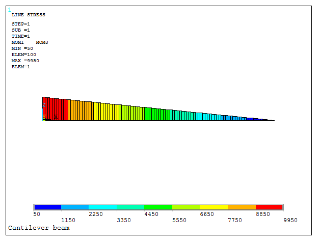
Figure 32. Bending moment diagram.