
PROBLEM
Figure 1 represents the model of a triangular support bracket. The thickness of this bracket is 4 mm. The material is laminated steel.
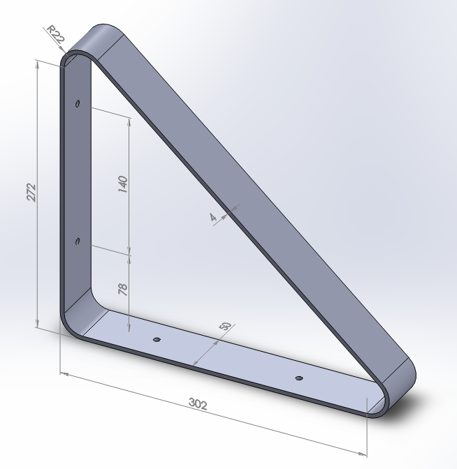
Figure 1. Triangular support bracket.
A force of 400 N acts on the bracket. Solve the problem for two loading conditions:
Table 1. Material properties.
| Laminated steel | |
| ESteel | 210 GPa |
| νSteel | 0.3 |
GEOMETRY OF THE MODEL
First of all, define the analysis type:
Main Menu > Preferences
Select "Structural".
Next, define the name for this particular problem, that is "Triangular support bracket" (Figure 2).
Utility Menu > File > Change Jobname
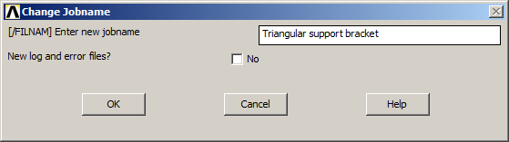
Figure 2. Change jobname for the problem.
Now, define the element type. This type of problem can be solved with SHELL elements. Select "Shell 8 node 281" (ANSYS HELP), as indicated in Figure 3.
Main Menu > Preprocessor > Element Type > Add/Edit/Delete
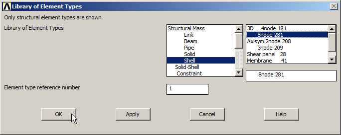
Figure 3. Element type: Shell 8 node 281.
For the material, define the mechanical properties (Figure 4).
Main Menu > Preprocessor > Material Props > Material Models
Define the material as "Structural – Linear – Elastic – Isotropic".
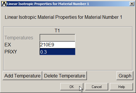
Figure 4. Material properties.
For the SHELL element, it is required to define the thickness (Figure 5).
Main Menu > Preprocessor > Sections > Shell > Lay-up > Add/Edit
Input 4 mm (0.004 m) in "Thickness".
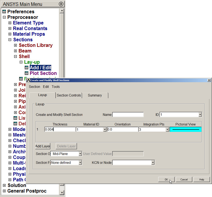
Figure 5. Defining the thickness for the SHELL element.
To create the geometry of the model, define a grid for the working plane (WP Settings), as indicated in Figure 6.
Utility Menu > WorkPlane > WP Settings …
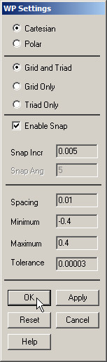
Figure 6. Working Plane Settings.
The grid can be displayed on the screen:
Utility Menu > WorkPlane > Display Working Plane
To create the geometry, the dimensions are referred to the midline. Table 2 shows the coordinates and radius of the circles.
Table 2. Coordinates for the circles.
| CIRCLE | X (m) | Y (m) | Radius (m) |
| 1 | 0.020 | 0.020 | 0.020 |
| 2 | 0.300 | 0.020 | 0.020 |
| 3 | 0.020 | 0.270 | 0.020 |
Create the three circles as indicated in Figure 7:
Main Menu > Preprocessor > Modeling > Create > Lines > Arcs > Full Circle
Look at the coordinates by clicking and dragging the cursor on the screen. Repeat this operation for each one of the circles.
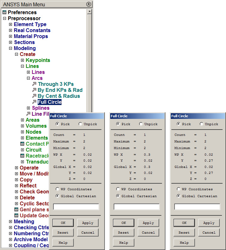
Figure 7. Creating three circles.
The circles are displayed on the screen (Figure 8).
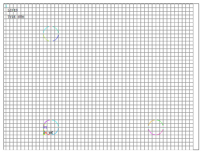
Figure 8. Graphic screen with the three circles.
After that, create two keypoints at the center of the top and right circles (Figure 9):
Main Menu > Preprocessor > Modeling > Create > Keypoints > On Working Plane
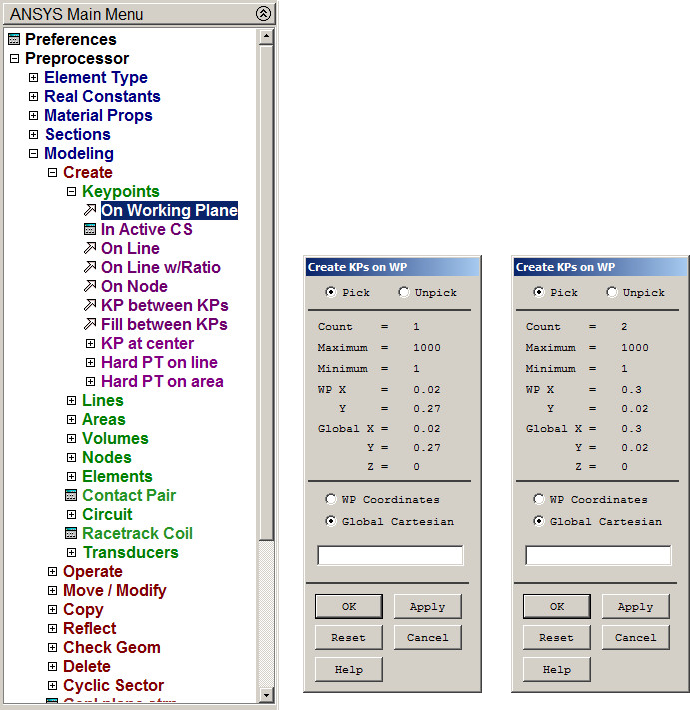
Figure 9. Creating two keypoints.
Figure 10 displays the circles and the keypoints. Number the keypoints:
Utility Menu > PlotCtrls > Numbering
And click "Keypoint numbers".
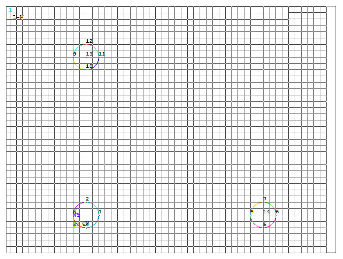
Figure 10. Keypoint numbers.
Now, align the working plane with the axis defined by the two keypoints, numbered as 13 and 14.
Utility Menu > WorkPlane > Align WP with > Keypoints +
Click the keypoints 13 and 14, and then "OK" (Figure 11).
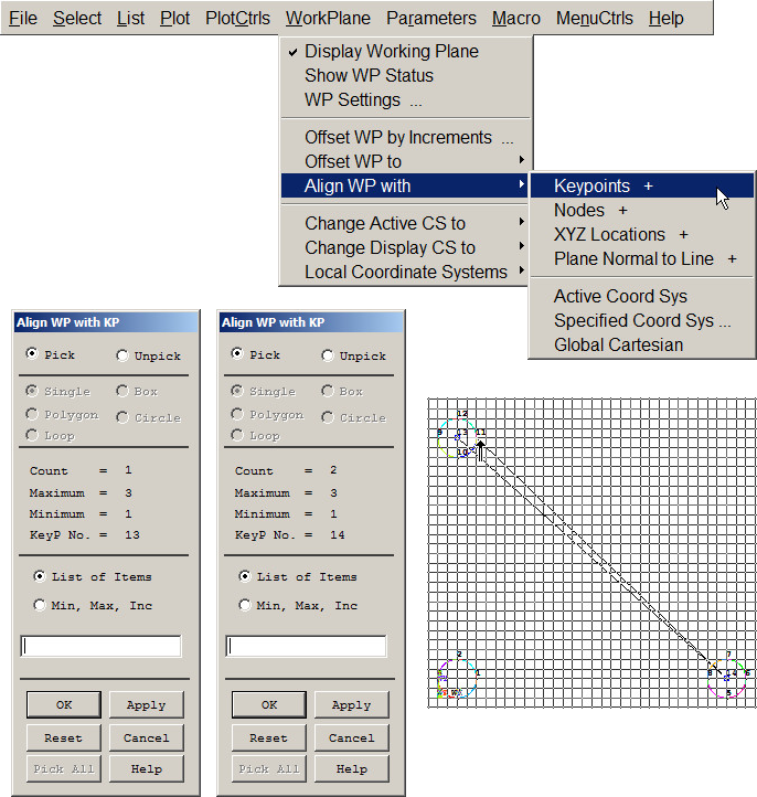
Figure 11. Align the working plane with the axis defined by two keypoints.
Figure 12 shows the graphic screen with the alignment of the working plane with the axis defined by the two keypoints.
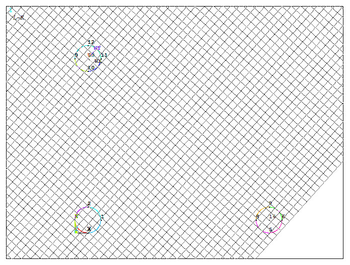
Figure 12. Graphic screen after "Align WP" operation.
Change the orientation of the working plane:
Utility Menu > WorkPlane > Offset WP by Increments …
Define 90 degrees and click "+Y", as indicated in Figure 13.
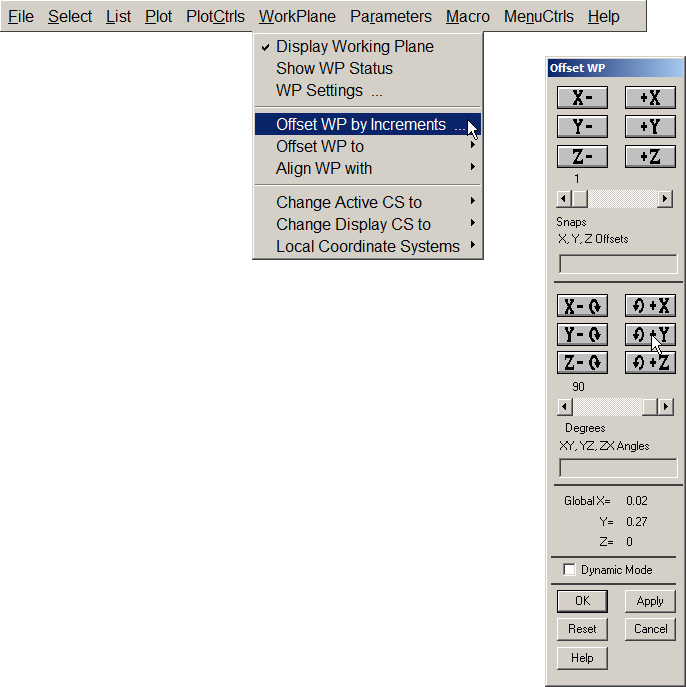
Figure 13. Applying "Offset WP by Increments".
Figure 14 shows the graphic screen after "Offset WP by Increments" operation.
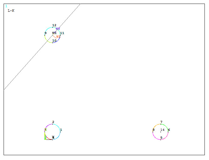
Figure 14. Graphic screen after "Offset WP by Increments".
Open the "Pan-Zoom-Rotate" tool:
Utility Menu > PlotCtrls > Pan Zoom Rotate
Click on "Box Zoom", as indicated in Figure 15 and expand a particular part of the model.
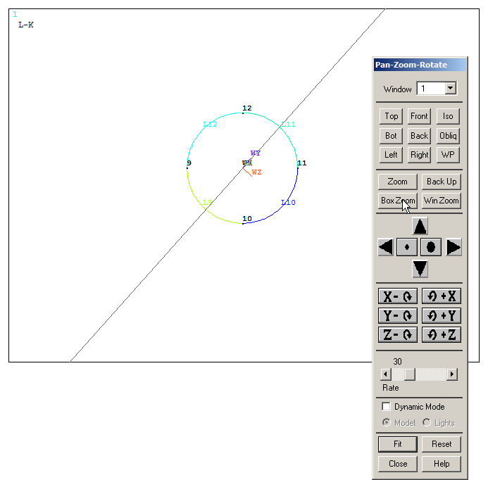
Figure 15. "Box Zoom" option.
Next, divide the circular line by the working plane in order to create the tangent point that is required to create the straight diagonal line (Figure 16).
Main Menu > Preprocessor > Modeling > Operate > Booleans > Divide > Line by WrkPlane
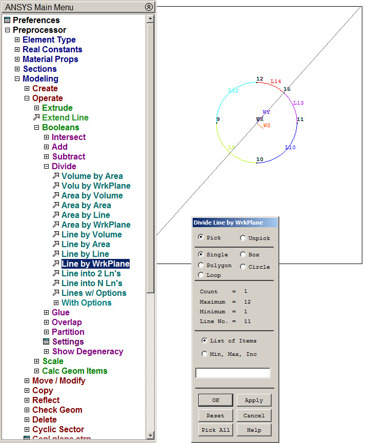
Figure 16. Divide Line by Working Plane.
Use "Fit view" button from "Pan-Zoom-Rotate" and repeat the same process for the circle on the right (Figure 17).
Utility Menu > WorkPlane > Offset WP to > Keypoints +
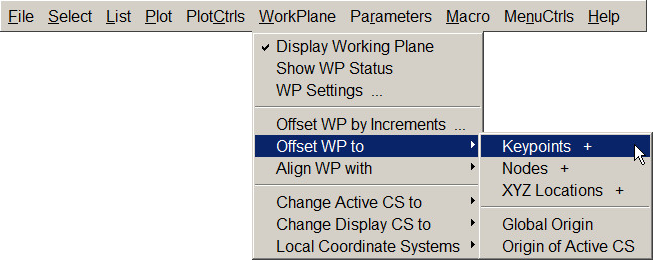
Figure 17. "Offset WP to Keypoints +".
Select the keypoint 14 and "OK". The working plane is displayed in Figure 18.
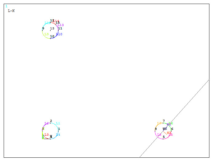
Figure 18. Changing Working Plane.
Dividing the line by the working plane, a new tangent point is created (Figure 19).
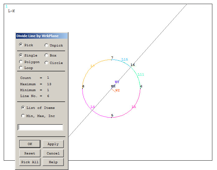
Figure 19. Divide Line by Working Plane.
Now, remove the lines that are not needed for the model (Figure 20):
Main Menu > Preprocessor > Modeling > Delete > Lines Only
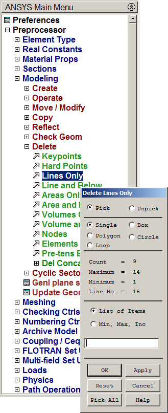
Figure 20. Delete "Lines Only".
Figure 21 represents the graphic screen selecting the lines to be deleted.
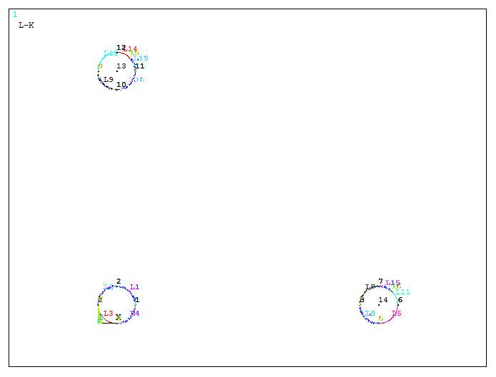
Figure 21. Deleting the lines.
Now, create the straight lines for the triangular support bracket.
Main Menu > Preprocessor > Modeling > Create > Lines > Straight Line
Figure 22 represents the keypoints and the lines.
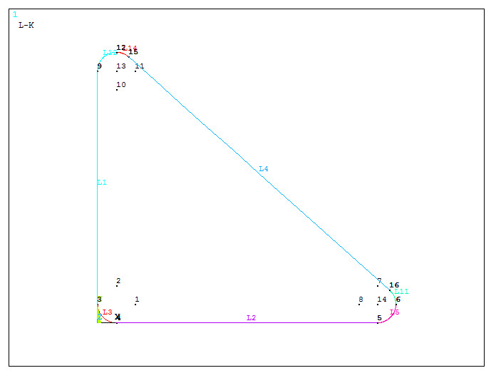
Figure 22. Created lines and keypoints.
Now, create two new keypoints to define the direction of the extrusion.
Main Menu > Preprocessor > Modeling > Create > Keypoints > In Active CS
Figure 23 shows the coordinates for the new keypoints.
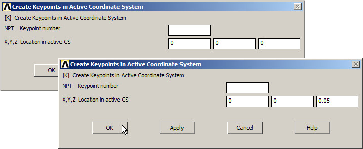
Figure 23. Creating two new keypoints.
Figure 24 displays a view with the lines and the new keypoints.
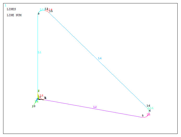
Figure 24. Lines with the new keypoints.
Create a line between these two keypoints.
Main Menu > Preprocessor > Modeling > Create > Lines > Straight Line
After that, extrude the triangular model (Figure 25).
Main Menu > Preprocessor > Modeling > Operate > Extrude > Lines > Along Lines
Select the lines that define the triangular model and "OK".
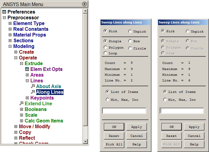
Figure 25. "Extrude Lines" operation.
Figure 26 represents the extruded model.
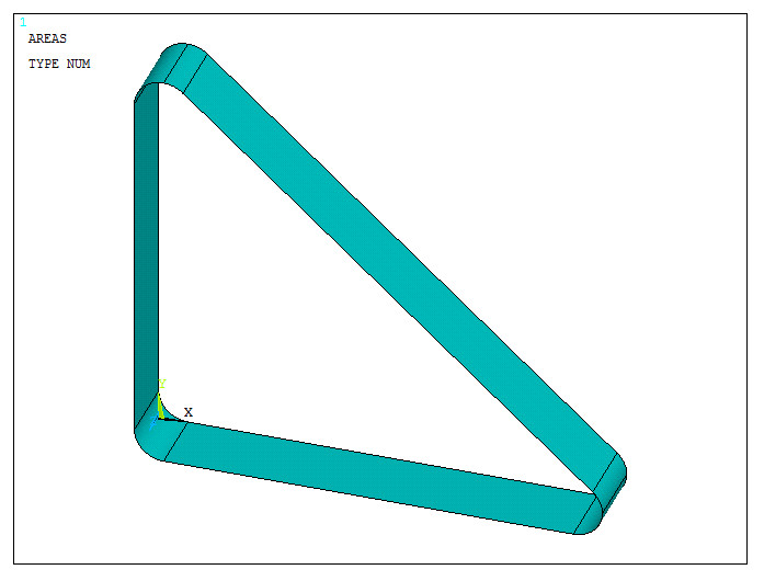
Figure 26. Extruded model.
Finally, create the circular holes on the vertical and horizontal sides of the bracket. First, align the working plane with keypoints (Figure 27).
Utility Menu > WorkPlane > Align WP with > Keypoints
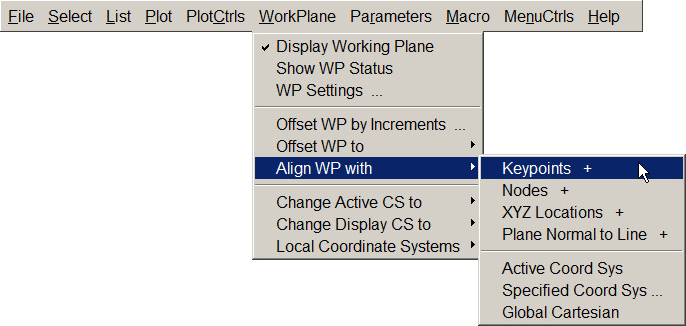
Figure 27. Align WP with keypoints.
For the new working plane, select keypoints 17 and 3 to define the vertical axis, and then click on keypoint 18 for the horizontal axis.
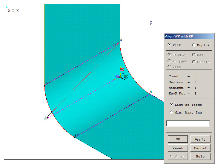
Figure 28. Aligning the working plane.
Create two circular areas on the vertical side (Figure 29).
Main Menu > Preprocessor > Modeling > Create > Areas > Circle > Solid Circle
The geometric characteristics of these circular areas are indicated in Table 3.
Table 3. Radius and coordinates for the circles.
| CIRCLES | X (m) | Y (m) | Radius (m) |
| 1 | 0.080 | 0.025 | 0.003 |
| 2 | 0.220 | 0.025 | 0.003 |
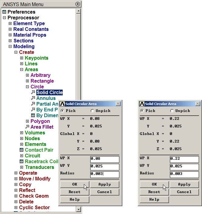
Figure 29. Creating circular areas on the vertical side.
Figure 30 displays the model with the two circular areas on the vertical side. Number areas from "Utility Menu – PlotCtrls – Numbering".
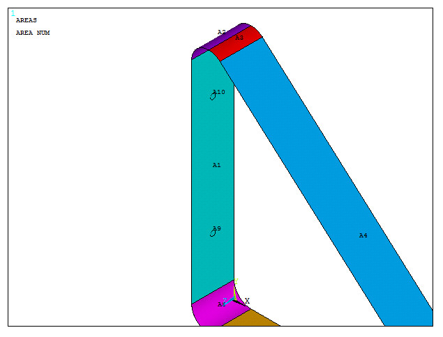
Figure 30. Numbered areas.
Subtract the two circular areas to create the holes:
Main Menu > Preprocessor > Modeling > Operate > Booleans > Subtract > Areas
Select all the areas, "OK" and then select the two circular areas and "OK".
Figure 31 represents the model with the circular holes on the vertical side.
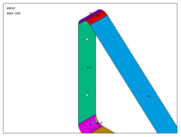
Figure 31. Circular holes on the vertical side.
Repeat the same operation to create the holes on the horizontal side of the bracket. First, align the working plane:
Utility Menu > WorkPlane > Align WP with > Keypoints
Select keypoints 17 and 4 for one axis, and the keypoint 18 for the other one (Figure 32).
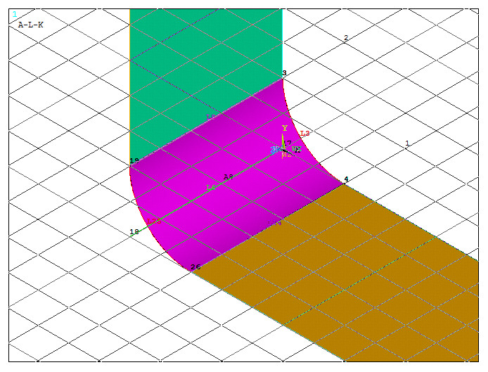
Figure 32. New orientation for the working plane.
As indicated in Figure 33, create two new circular areas.

Figure 33. Creating circular areas on the horizontal side.
Figure 34 shows the two circular areas on the horizontal side.
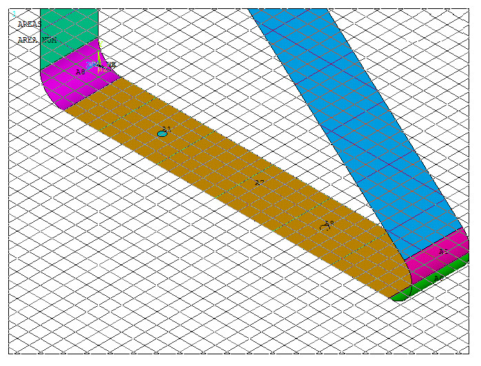
Figure 34. Circular areas on the horizontal side.
Again, subtract these circular areas as described before (Figure 35).
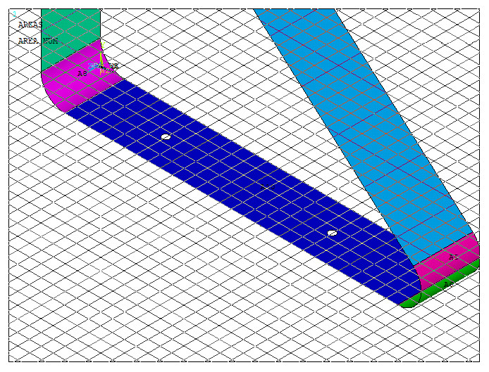
Figure 35. Circular holes on the horizontal side.
Figure 36 represents the model of the triangular support bracket.
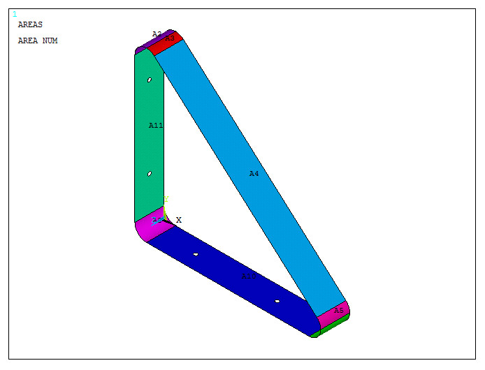
Figure 36. Model of the triangular support bracket.
With the geometry completely defined, mesh the model. Define an element size of 4 mm (Figure 37).
Main Menu > Preprocessor > Meshing > Size Cntrls > Manual Size > Areas > All Areas
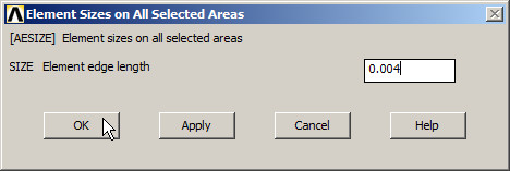
Figure 37. Element size (4 mm).
Finish the meshing process:
Main Menu > Preprocessor > Meshing > Mesh > Areas > Free
Click "Pick All".
Figure 18 represents the meshed model.
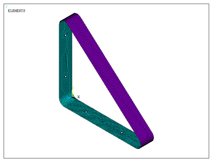
Figure 38. Meshed model.
The model can be displayed with the thickness by means of "Size and Shape" option:
Utility Menu > PlotCtrls > Style > Size and Shape
Activate "On" from ESHAPE. Figure 39 shows the scaled model.
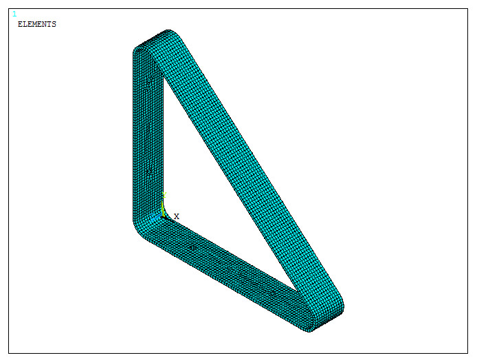
Figure 39. Meshed model with "ESHAPE" option.
LOADS AND BOUNDARY CONDITIONS
For the first loading condition, the triangular support bracket is supposed to be attached to the wall through the holes on the vertical side. So, restrict all degrees of freedom on the lines that define the circular holes (Figure 40).
Main Menu > Preprocessor > Loads > Define Loads > Apply > Structural > Displacement > On Lines
Select the corresponding lines and "All DOF".
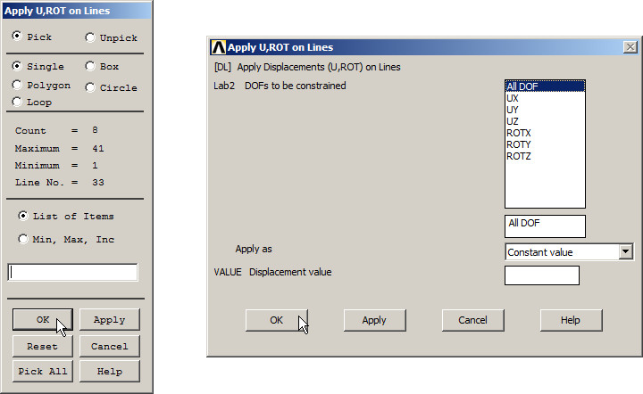
Figure 40. "All DOF" on the vertical holes.
To simulate the load acting on the shelf, apply a force of 400 N distributed on the 8 keypoints that define the horizontal holes.
Main Menu > Preprocessor > Loads > Define Loads > Apply > Structural > Force/Moment > On Keypoints
Input a value of -400/8 for each keypoint in the FY direction (Figure 41).
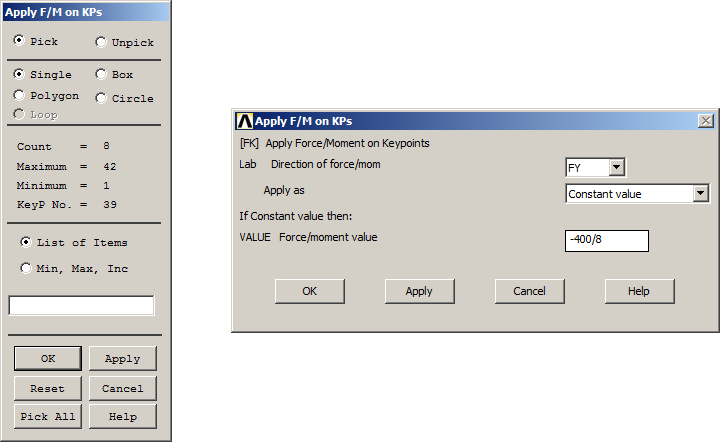
Figure 41. Applying forces on Keypoints.
Figure 42 shows the model with the loads and boundary conditions for the first loading condition.
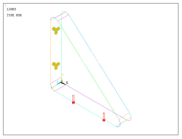
Figure 42. First loading condition on the model.
Save the first loading condition.
Main Menu > Solution > Load Step Opts > Write LS File
Save it as "1" (Figure 43).

Figure 43. Save the first loading condition.
For the second loading condition, the bracket is supposed to be located below the shelf. Assume a pressure acting on the horizontal side. First, delete the previously defined load (Figure 44).
Main Menu > Preprocessor > Loads > Define Loads > Delete > Structural > Force/Moment > On Keypoints
Click "Pick All".
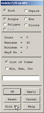
Figure 44. Delete forces of the first loading condition.
Since the pressure is distributed on the area, first check the value of the corresponding area from "Picked Entities".
Utility Menu > List > Picked Entities
In "Model Query Picker", select "Area" and "OK" (Figure 45). In the window "Measurements of Area" appears the value of 0.0139435 m2. The window "ASUM Command" details the geometric properties of the selected area.
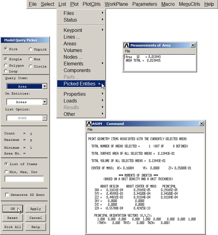
Figure 45. Checking the area with "Picked Entities".
So, the value of the pressure is 400/0.0139435 Pa, as indicated in Figure 46.
Main Menu > Preprocessor > Loads > Define Loads > Apply > Structural > Pressure > On Areas
Apply the pressure on the below part.
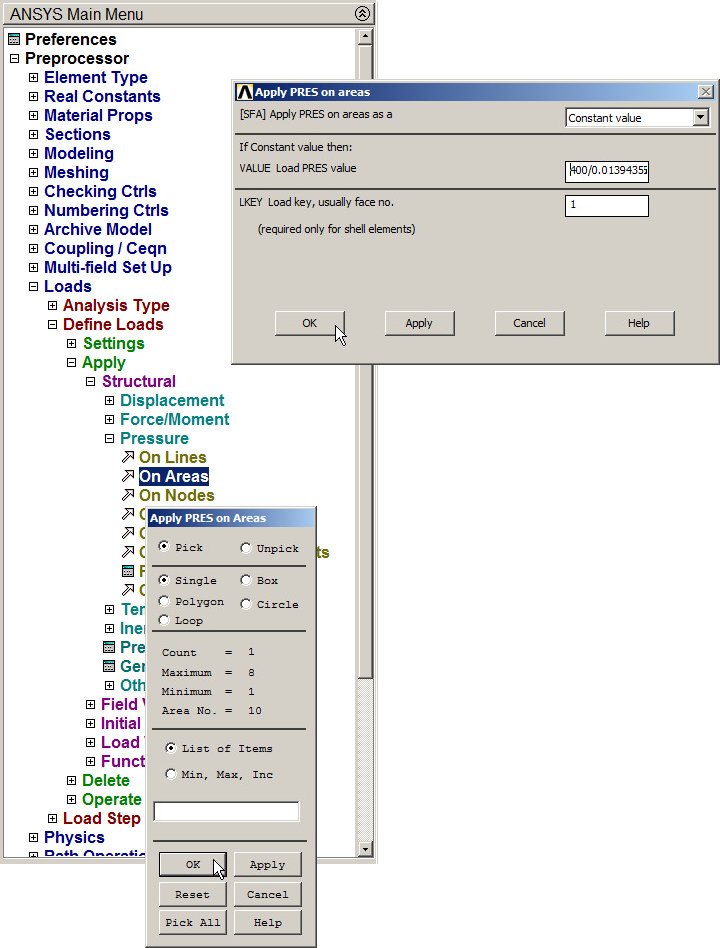
Figure 46. Applying the pressure on the area.
The second loading condition is displayed in Figure 47. The pressure is represented by a red arrow in the center of the area.
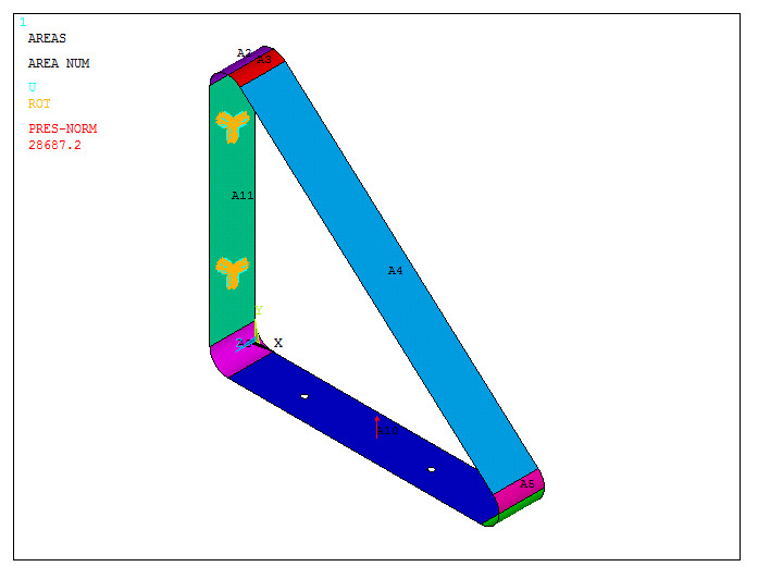
Figure 47. Second loading condition on the model.
Save the second loading condition as "2" (Figure 48).
Main Menu > Solution > Load Step Opts > Write LS File
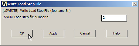
Figure 48. Save the second loading condition.
SOLUTION
Solve the problem taking into account the two loading conditions:
Main Menu > Solution > Solve > From LS Files
Define "1" for LSMIN and "2" for LSMAX, as indicated in Figure 49.
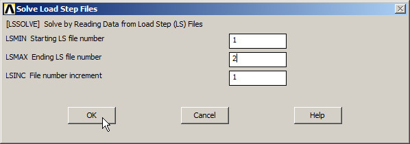
Figure 49. Solve the problem for the two loading conditions.
RESULTS
Evaluate the stress distribution in the model. Select "von Mises stress" (Figure 50).
Main Menu > General Postproc > Plot Results > Contour Plot > Nodal Solu
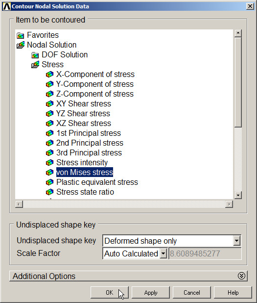
Figure 50. "von Mises stress".
To evaluate the results for the two loading conditions:
Main Menu > General Postproc > Read Results
Select "First Set" for the first loading condition and "Next Set" for the second one. Each time use "Plot Results" option.
Figures 51 and 52 represent the stress distribution for the first and second loading conditions, respectively.

Figure 51. Results for the first loading condition.
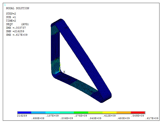
Figure 52. Results for the second loading condition.