
PROBLEM
Figure 1 represents a model of a tin made of aluminium. Find out the appropriate thickness for this particular model. The dimensions are referred to the midline.
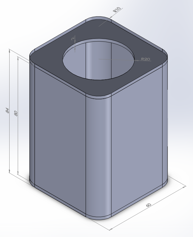
Figure 1. Tin model.
Solve the problem for two loading conditions:
Table 1 indicates the mechanical properties of the aluminium.
Table 1. Material properties.
| Aluminium 6061 T6 | |
| EAluminium | 69 GPa |
| Sy Aluminium | 275 MPa |
| νAluminium | 0.33 |
GEOMETRY OF THE MODEL
First of all, define the analysis type:
Main Menu > Preferences
Activate the "Structural" option.
Now, change the jobname for this particular problem: "Tin" (Figure 2).
Utility Menu > File > Change Jobname
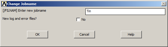
Figure 2. Change the jobname: "Tin".
Next, choose the element type. Select "Shell 8 node 281" (ANSYS HELP), as indicated in Figure 3.
Main Menu > Preprocessor > Element Type > Add/Edit/Delete
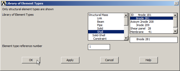
Figure 3. Element type: "Shell 8 node 281".
Input the mechanical properties of the material.
Main Menu > Preprocessor > Material Props > Material Models
Define the material as "Structural – Linear – Elastic – Isotropic".
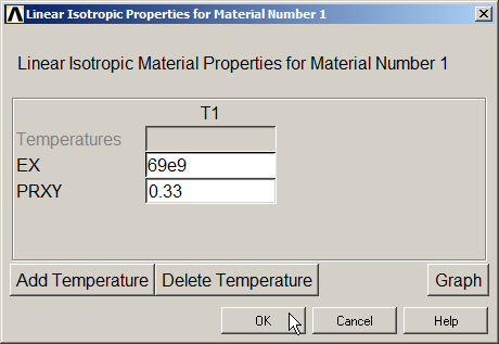
Figure 4. Material properties.
For this type of element, define the value of the thickness:
Main Menu > Preprocessor > Sections > Shell > Lay-up
Figure 5 displays the definition of the thickness (0.001 m).
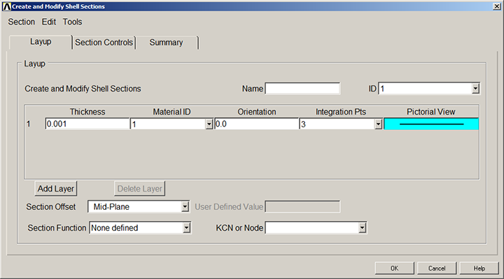
Figure 5. Thickness for the "Shell" element.
Now, create a grid for the working plane.
Utility Menu > WorkPlane > WP Settings …
Figure 6 shows the parameters for the grid.
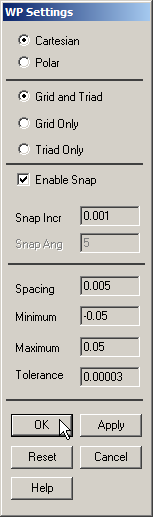
Figure 6. Parameters for the grid.
Display the grid on the screen with the option "Display Working Plane" from the "Utility Menu".
After that, create the four keypoints at the bottom of the tin (Figure 7). Table 2 indicates the coordinates for these keypoints.
Table 2. Coordinates of the keypoints at the bottom.
| KEYPOINTS | X (m) | Y (m) |
| 1 | -0.03 | -0.03 |
| 2 | -0.03 | 0.03 |
| 3 | 0.03 | 0.03 |
| 4 | 0.03 | -0.03 |
Main Menu > Preprocessor > Modeling > Create > Keypoints > On Working Plane
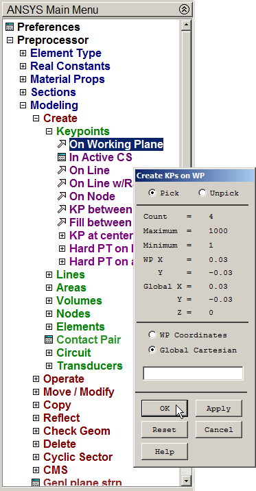
Figure 7. Creating keypoints.
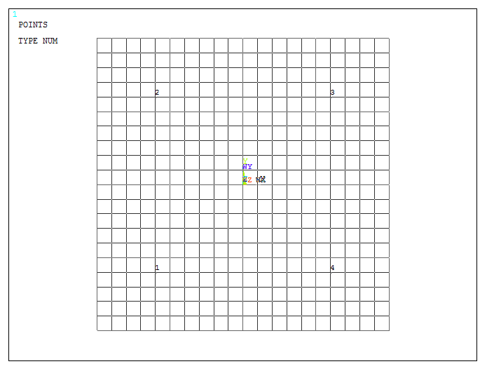
Figure 8. Graphic screen with the four keypoints at the bottom.
Next, create the lines that join the keypoints.
Main Menu > Preprocessor > Modeling > Create > Lines > Straight Line
Click on the keypoints consecutively. Figure 9 represents the lines for the basis of the tin.
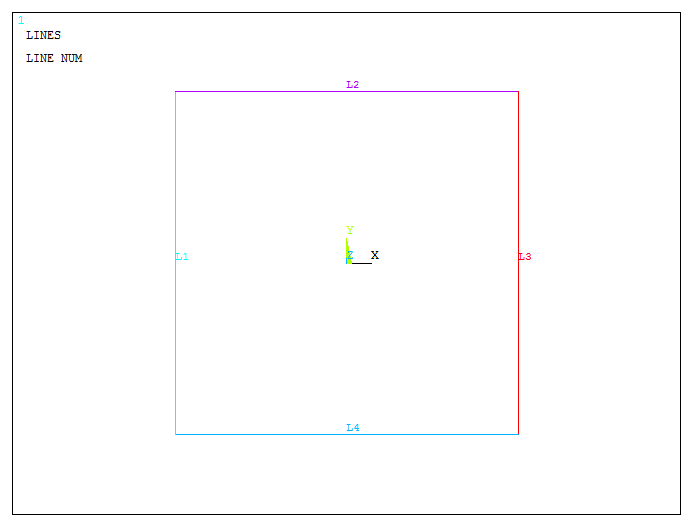
Figure 9. Graphic screen with the four lines for the basis.
For the curvature at the corners, apply the "Line Fillet" option.
Main Menu > Preprocessor > Modeling > Create > Lines > Line Fillet
Selecting two lines and "Apply", define a fillet radius of 0.01 m, as indicated in Figure 10.
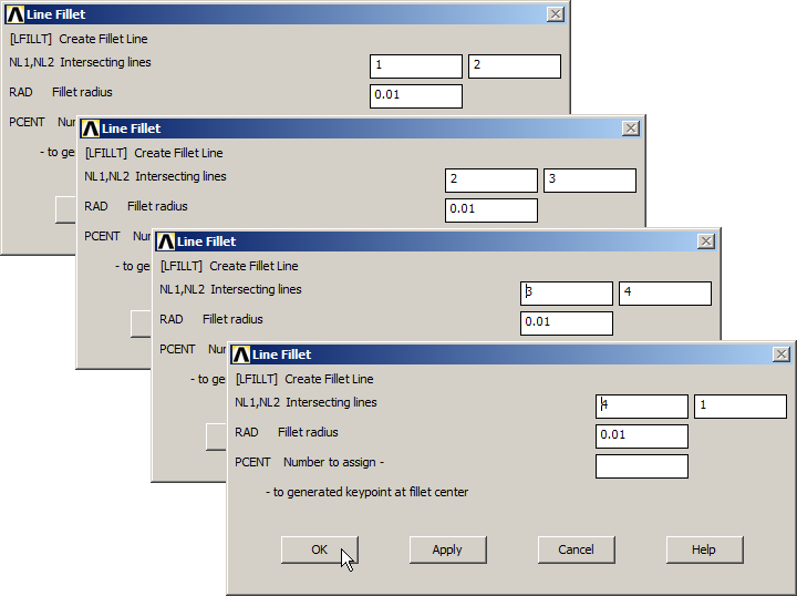
Figure 10. "Line Fillet" operation for the curvatures at the corners.
To change the view of the model:
Utility Menu > PlotCtrls > View Settings > Viewing Direction
And define the parameters indicated in Figure 11.
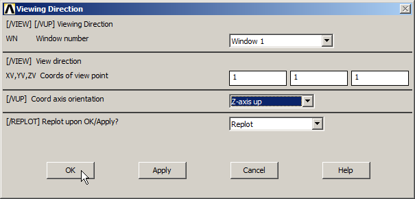
Figure 11. "Viewing Direction" option.
Figure 12 displays the new view.
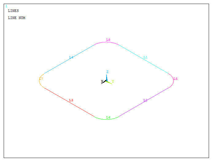
Figure 12. New orientation for the model.
Now, create four keypoints to define the direction of the extrusion (Figure 13):
Main Menu > Preprocessor > Modeling > Create > Keypoints > In Active CS

Figure 13. Creating four new keypoints.
With these keypoints, create three straight lines, so that when extruding, there will be three different parts: the main body, the upper part and the lower part. Figure 14 shows the new four keypoints.
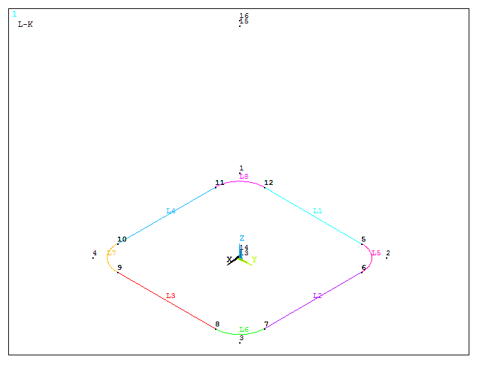
Figure 14. Creating keypoints to define the direction of the extrusion.
Then, create the three straight lines:
Main Menu > Preprocessor > Modeling > Create > Lines > Lines > Straight Line
Figure 15 displays the lines that define the direction of the extrusion.
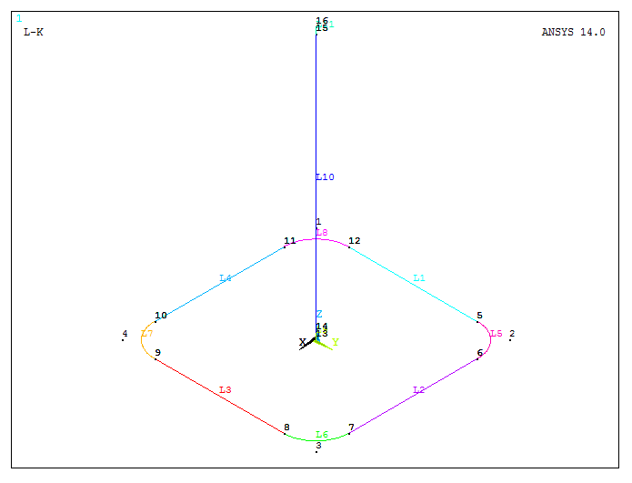
Figure 15. Lines for the direction of the extrusion.
Now, extrude the lines at the bottom of the tin.
Main Menu > Preprocessor > Modeling > Operate > Extrude > Lines > Along Lines
Select the lines at the bottom, click "OK", and then select the three vertical straight lines, as indicated in Figure 16.
Remind that all the instructions appear at the bottom left in the "PROMPT USER INFO".
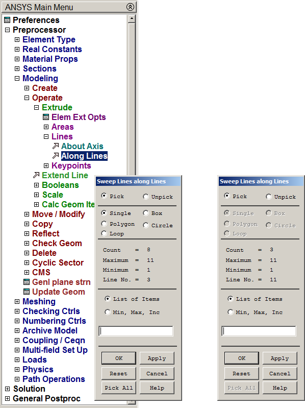
Figure 16. Selecting the lines for the extrusion.
After "Extrude" operation, the model is represented in Figure 17.
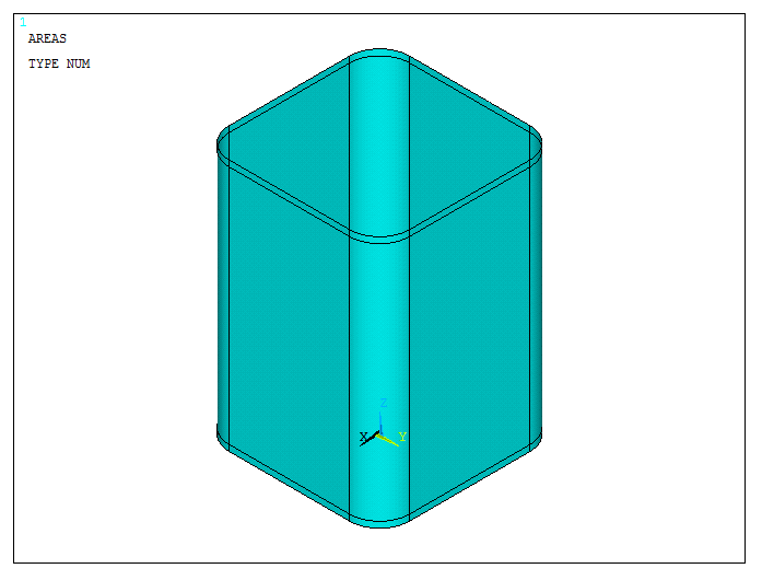
Figure 17. Model after "Extrude" operation.
Figure 18 represents the model with the numbered lines:
Utility Menu > Plot > Lines
For numbering the lines:
Utility Menu > PlotCtrls > Numbering
And activate "Line numbers".
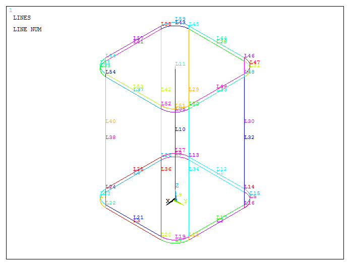
Figure 18. Model with the numbered lines.
After that, create the areas at the bottom and at the top. First, select the lines located at 0.002 m in Z-axis (Figure 19).
Main Menu > Preprocessor > Modeling > Create > Areas > Arbitrary > By Lines
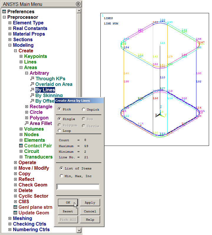
Figure 19. Selecting the lines to define the area at the bottom.
Click "OK" and the area is created as represented in Figure 20.
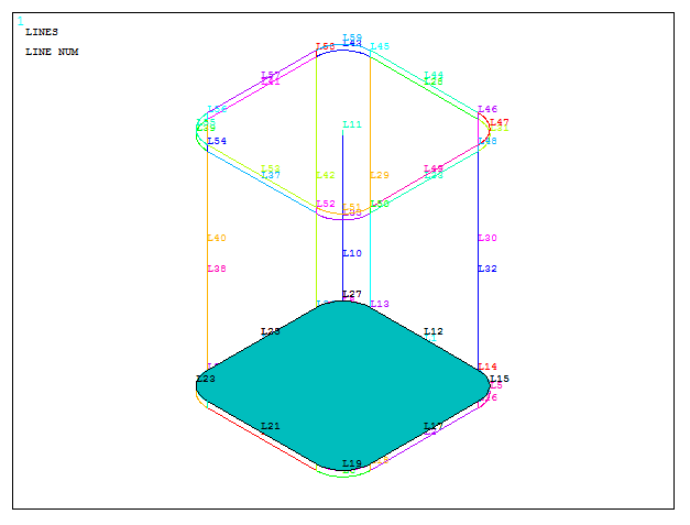
Figure 20. Area at the bottom.
In the same way, create the area at the top. The lines are located at 0.082 m in Z-axis (Figure 21).
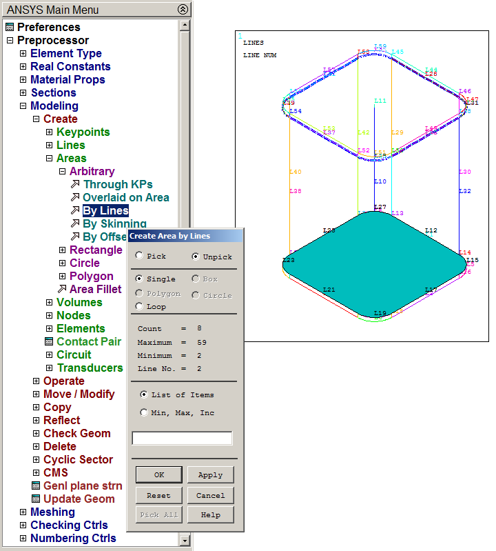
Figure 21. Selecting the lines to define the area at the top.
After that, the model is represented in Figure 22.
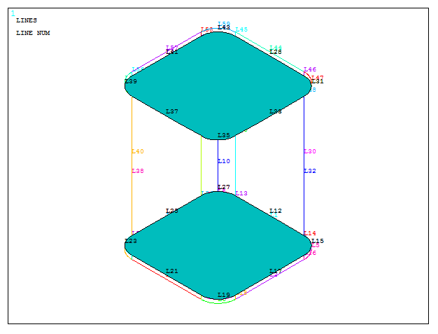
Figure 22. Areas at the bottom and at the top of the model.
Disable the numbers of the lines and apply "Multi-Plots".
Utility Menu > Plot > Multi-Plots
Figure 23 shows the model of the tin.
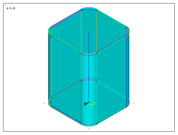
Figure 23. "Multi-Plots" options.
Now, create a circular area at the top of the tin. First, move the working plane:
Utility Menu > WorkPlane > Offset WP to Keypoints +
Select keypoint 15 and the working plane is moved as displayed in Figure 24.
Number the areas.
Utility Menu > PlotCtrls > Numbering
And activate "Area numbers".
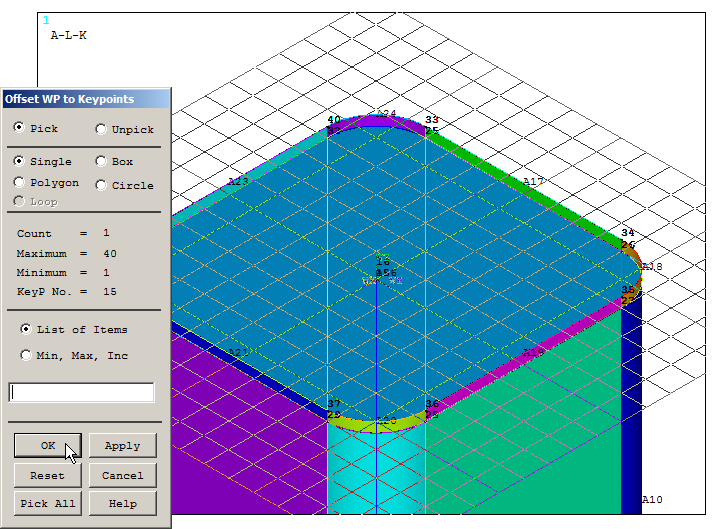
Figure 24. Working Plane at the top of the model.
Now, create the circle with a radius of 0.02 m (Figure 25).
Main Menu > Preprocessor > Modeling > Create > Areas > Circle > Solid Circle
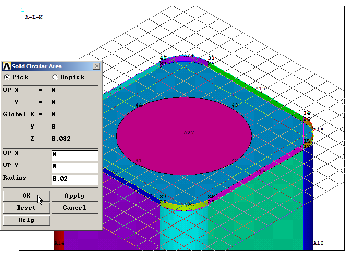
Figure 25. Creating the circular area.
Subtract this circular area to create the hole.
Main Menu > Preprocessor > Modeling > Operate > Booleans > Subtract > Areas
First, select the total area at the top of the model, "OK" and then select the circular area, as indicated in Figure 26. After that, move again the working plane 2 mm down.
Utility Menu > WorkPlane > Offset WP by Increments
Input the coordinates (0, 0, -0.002).
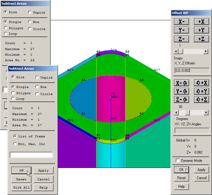
Figure 26. "Subtract Areas" operation.
Now, divide the vertical line through the working plane in its new position.
Main Menu > Preprocessor > Modeling > Operate > Booleans > Divide > Line by WrkPlane
And select line 10, as indicated in Figure 27.
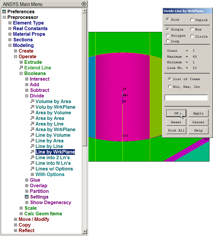
Figure 27. Dividing the line by the working plane.
Extrude the four lines that define the circle along the 2 mm straight line (Figure 28).
Main Menu > Preprocessor > Modeling > Operate > Extrude > Lines > Along Lines
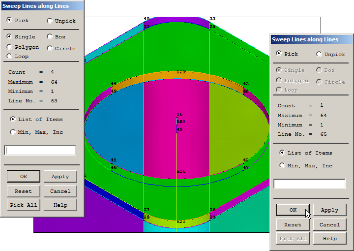
Figure 28. Extruding the lines that define the circular hole.
With the geometry completely defined, mesh the model defining an element size of 4 mm (Figure 29).
Main Menu > Preprocessor > Meshing > Size Cntrls > Manual Size > Areas > All Areas
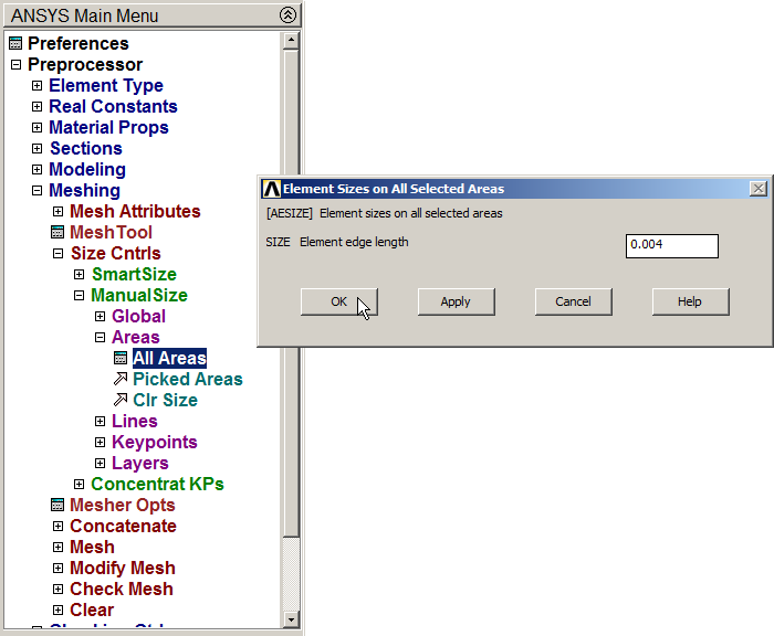
Figure 29. Defining the element size.
Finish the meshing process. Figure 30 displays the meshed model:
Main Menu > Preprocessor > Meshing > Mesh > Areas > Free
And click "Pick All".
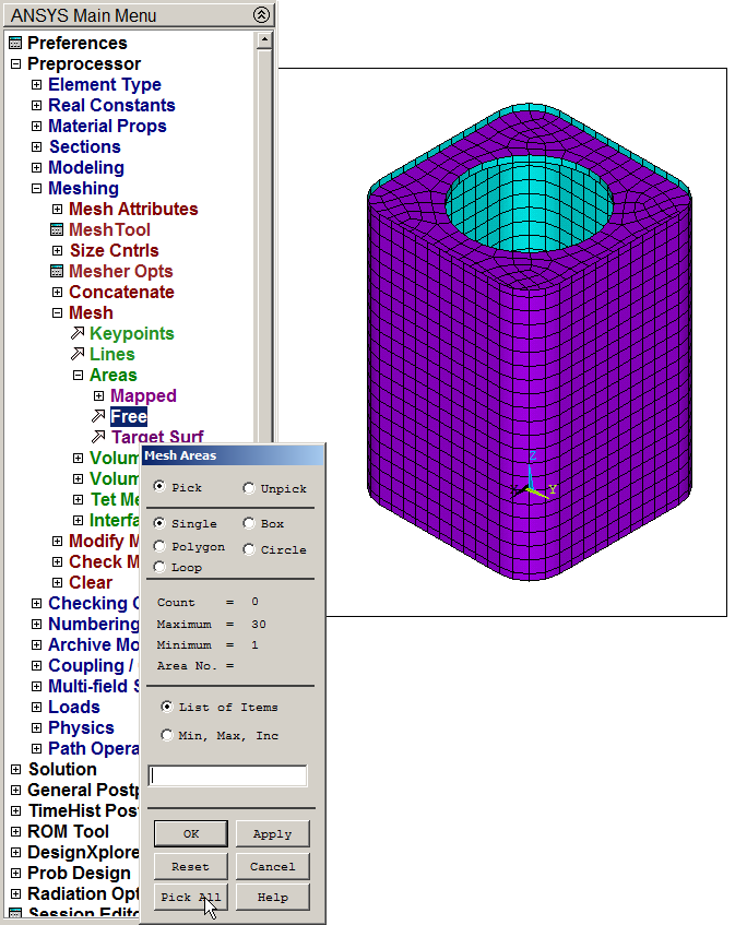
Figure 30. Meshed model.
LOADS AND BOUNDARY CONDITIONS
For this particular model, restrict the vertical displacements in Z direction. This restriction is applied on the lines at the bottom of the model (Figure 31).
Display the lines from "Utility Menu – Plot – Lines". Then:
Main Menu > Preprocessor > Loads > Define Loads > Apply > Structural > Displacement > On Lines
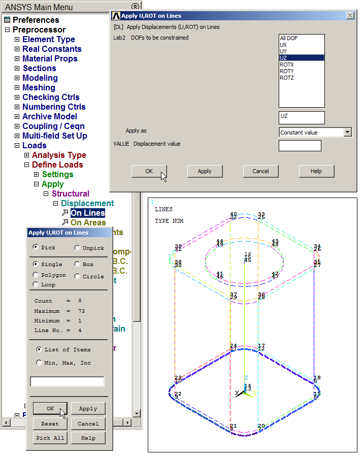
Figure 31. Restriction on the lines at the bottom in UZ direction.
Figure 32 represents the graphic screen with the restrictions on the lines at the bottom.
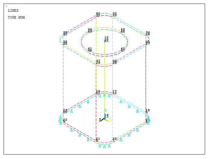
Figure 32. Graphic screen with the restrictions on the lines.
Moreover, two keypoints at the basis (5 and 12) have to be restricted in UX and UZ directions and rotation ROTY, as indicated in Figure 33.
Main Menu > Preprocessor > Loads > Define Loads > Apply > Structural > Displacement > On Keypoints
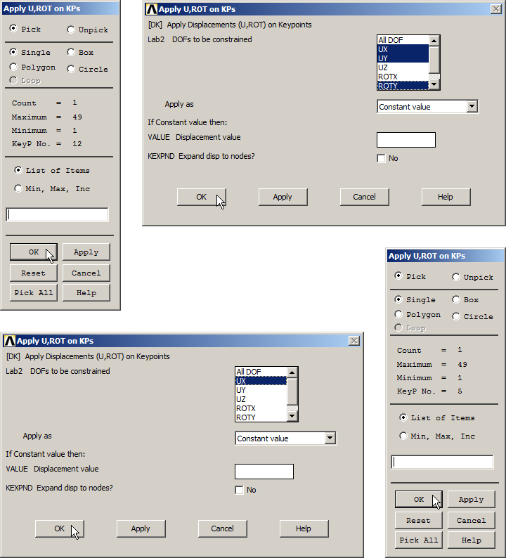
Figure 33. Restrictions at the keypoints 5 and 12.
Now, for the first loading condition, apply a force of 1500 N at the top of the model, that simulates the stacking.
Since this force is applied to the nodes located at the top, select these nodes:
Utility Menu > Select > Entities …
First, select the lines at the top with the option "By Num/Pick" (Figure 34).
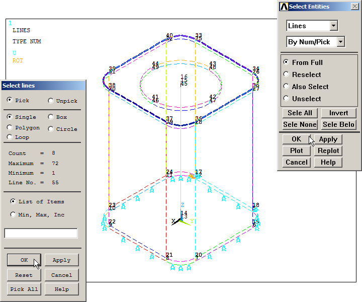
Figure 34. Selecting the lines at the top.
Again, from "Select Entities", select the nodes attached to lines, as indicated in Figure 35. Now, "Utility Menu – Plot – Nodes".
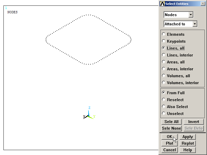
Figure 35. "Select Entities" for the nodes.
Apply the force:
Main Menu > Preprocessor > Loads > Define Loads > Apply > Structural > Force/Moment > On Nodes
Click on "Box" and drag the mouse to select the nodes. As observed in Figure 36 there are 112 nodes.
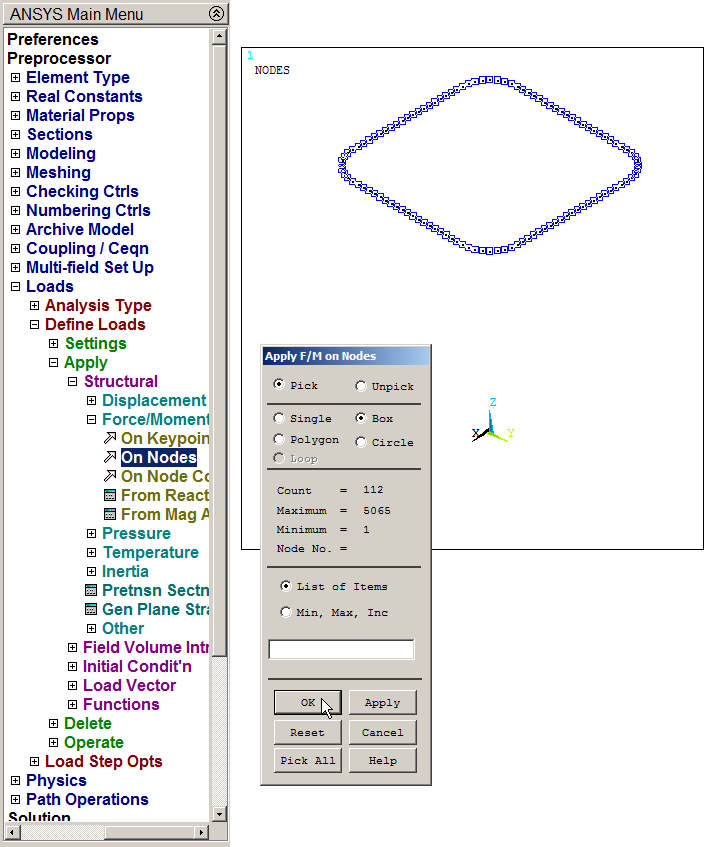
Figure 36. Applying forces "On Nodes".
To apply the force in each node, it has to be distributed among the 112 nodes, as indicated in Figure 37.
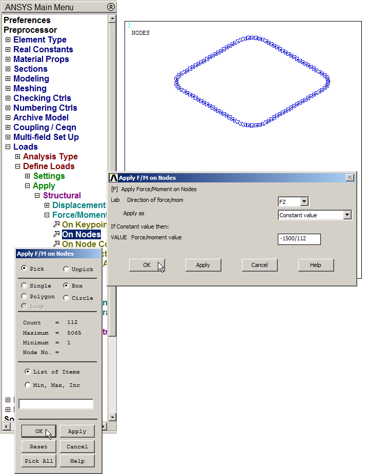
Figure 37. Applying the force in FZ direction.
Now, it is very important to select all the geometric entities (Figure 38).
Utility Menu > Select > Everything
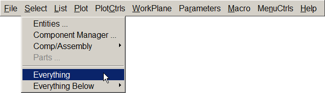
Figure 38. Select all the geometric entities.
Applying "Multi-Plots", Figure 39 represents the model with the loads and the boundary condition.
Utility Menu > Plot > Multi-Plots
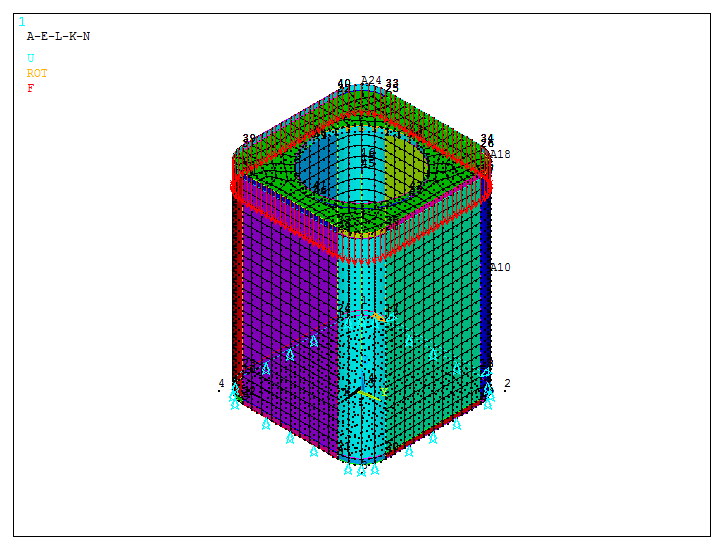
Figure 39. Model for the first loading condition.
Save the first loading condition:
Main Menu > Preprocessor > Solution > Load Step Opts > Write LS File
Input number "1" for this loading condition, as indicated in Figure 40.
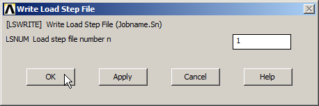
Figure 40. Save the first loading condition.
Now, before defining the second loading condition, the forces have to be deleted:
Main Menu > Preprocessor > Loads > Define Loads > Delete > Structural > Force/Moment > On Nodes
And click "Pick All".
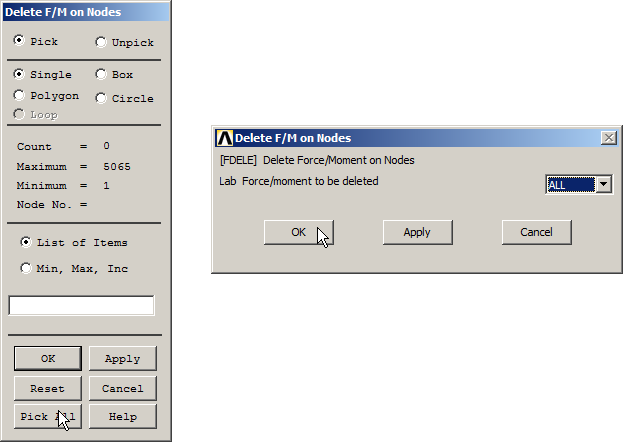
Figure 41. Delete the forces for the first loading condition.
To define the second loading condition, repeat the process from "Select Entities" in order to select the lines that define the circle in which a load of 100 N is acting.
Figures 42, 43 and 44 represent the process.
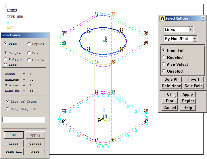
Figure 42. Select the lines of the circular hole.
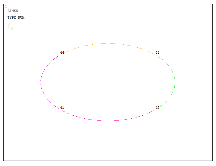
Figure 43. Graphic screen with the selected circular lines.
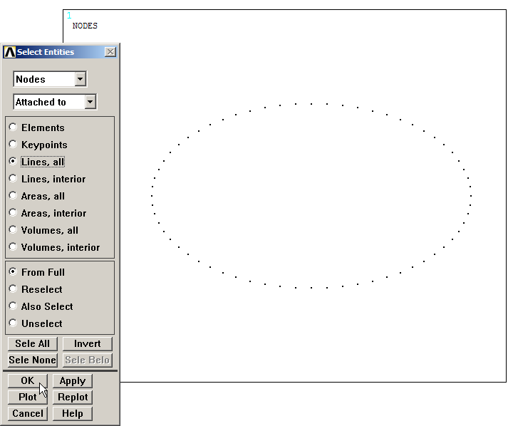
Figure 44. Graphic screen with the nodes of the circular line.
As observed in Figure 45, there are 64 nodes. So, the force has to be distributed on these nodes with a value of -100/64 N.
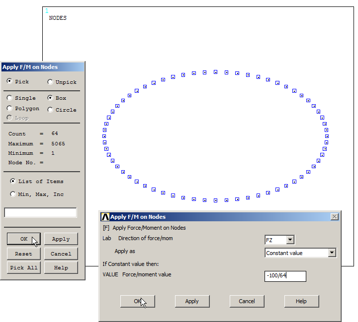
Figure 45. Applying the force on the nodes.
Figure 46 represents the forces acting on the nodes.
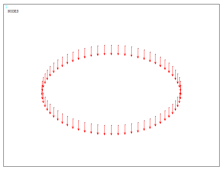
Figure 46. Applied forces on the nodes.
Again, select all the geometric entities.
Utility Menu > Select > Everything
And save the second loading condition, as indicated in Figure 47.
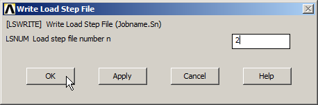
Figure 47. Save the second loading condition.
SOLUTION
Solve the problem taking into account the two loading conditions:
Main Menu > Solution > Solve > From LS Files
Define the calculation as indicated in Figure 48.
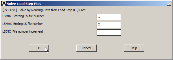
Figure 48. Solve the problem for the two loading conditions.
Figure 49 displays the model after "Solution is done!".
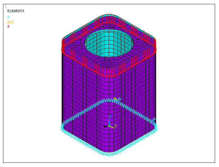
Figure 49. Solved model for the first loading condition.
RESULTS
Analyze the results.
First, evaluate the external reactions at the bottom of the model.
Main Menu > General Postproc > List Results > Reaction Solu
Figure 50 displays the reactions for the first loading condition.
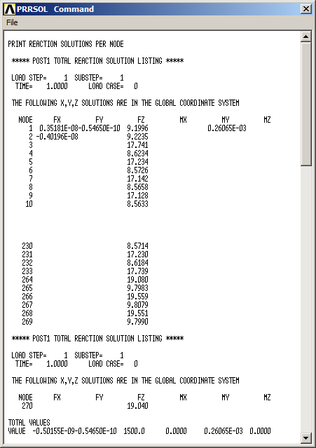
Figure 50. External reactions for the first loading condition.
For the stress distribution:
Main Menu > General Postproc > Read Results > First Set
Then:
Main Menu > General Postproc > Plot Results > Contour Plot > Nodal Solu
And select "von Mises stress". Figure 51 represents the stress distribution for the first loading condition.
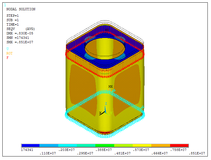
Figure 51. Stress distribution for the first loading condition.
Now, Figure 52 shows the solved model for the second loading condition.
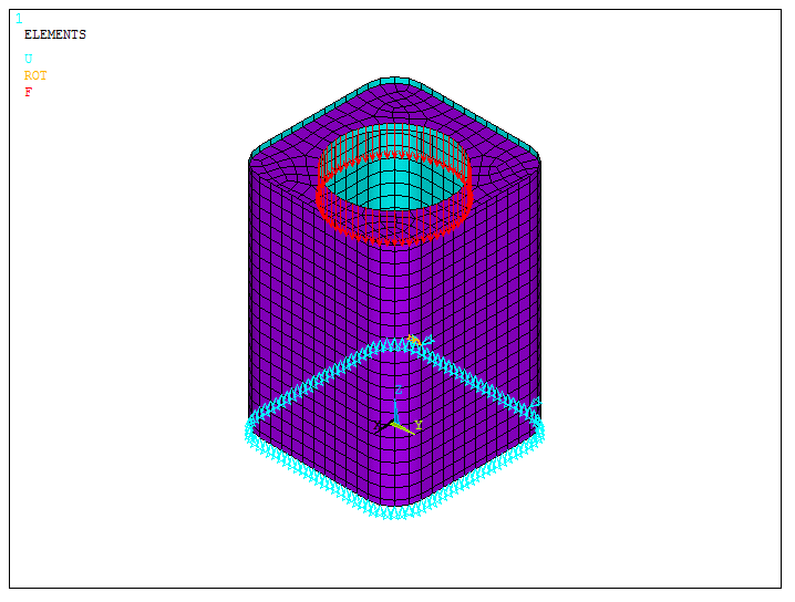
Figure 52. Solved model for the second loading condition.
To obtain the results for the second loading condition:
Main Menu > General Postproc > Read Results > Next Set
In the same way as explained before, obtain the results for the external reactions (Figure 53).
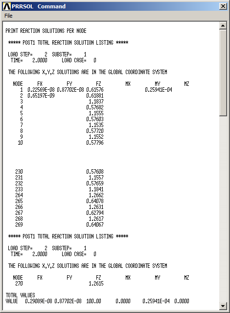
Figure 53. External reactions for the second loading condition.
Figure 54 represents the stress distribution for the second loading condition.
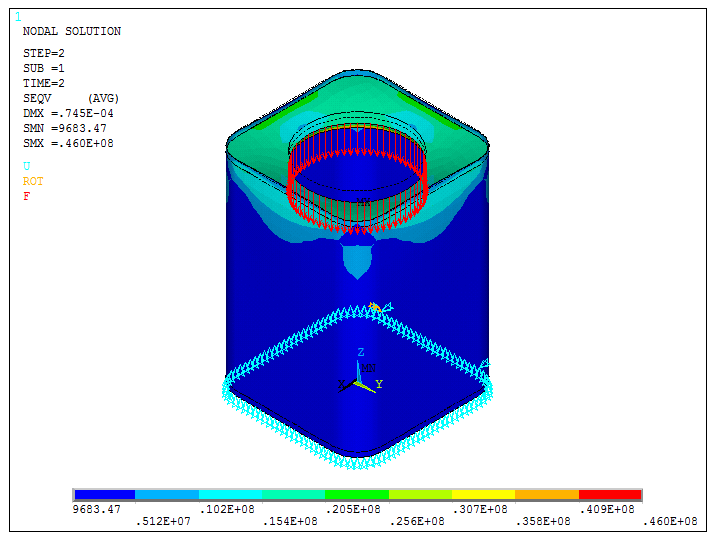
Figure 54. Stress distribution for the second loading condition.
Finish the problem by checking the results for different thicknesses. First, define a thickness of 0.3 mm.
Main Menu > Preprocessor > Sections > Shell > Lay-up > Add/Edit
Figure 55 displays the window to define the new value of the thickness.
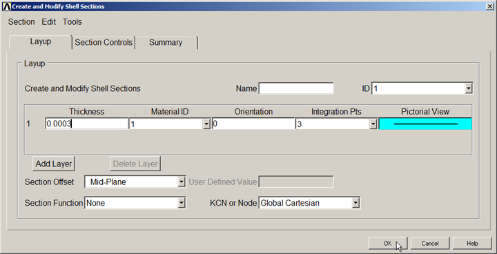
Figure 55. Modifying the thickness.
Figure 56 shows the results for the second loading condition and a thickness of 0.3 mm.
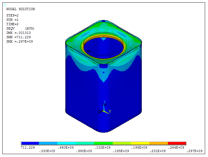
Figure 56. Results for the second loading condition and 0.3 mm thickness.
Finally, Figure 57 shows the results for a thickness of 0.4 mm.
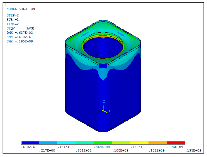
Figure 57. Results for the second loading condition and 0.4 mm thickness.