PROBLEM
Figure 1a shows an aluminium pressure tank. A pressure of 5 bar is acting on the walls of this pressure tank.
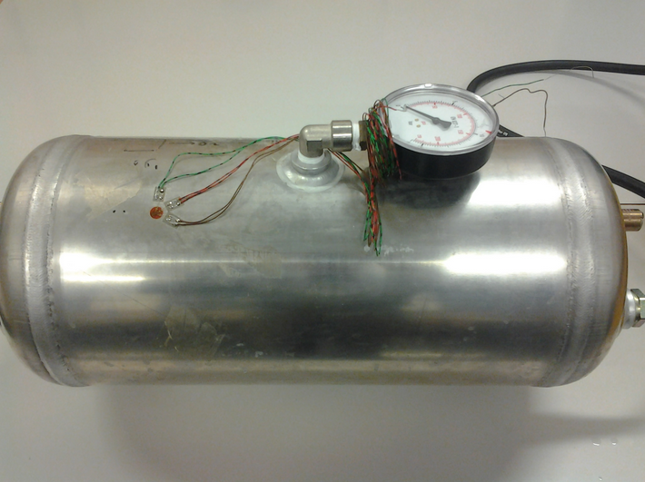
Figure 1a. Pressure tank.
Figure 1b represents the model with the dimensions of the pressure tank. The thickness of the walls is 3 mm. The dimensions are referred to the midline.
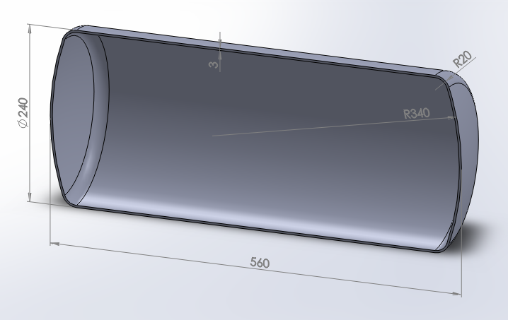
Figure 1b. Dimensions of the pressure tank (wall thickness: 3 mm).
Table 1 indicates the material properties of the aluminium.
Table 1. Material properties.
| Aluminium | |
| EAluminium | 73 GPa |
| Sy Aluminium | 250 MPa |
| νAluminium | 0.33 |
GEOMETRY OF THE MODEL
First of all, define the analysis type:
Main Menu > Preferences
And select "Structural".
Change the jobname for this particular problem, that is "Pressure tank".
Utility Menu > File > Change Jobname
After that, select the element type for the problem: "Shell 8 node 281" (ANSYS HELP), as indicated in Figure 2.
Main Menu > Preprocessor > Element Type > Add/Edit/Delete
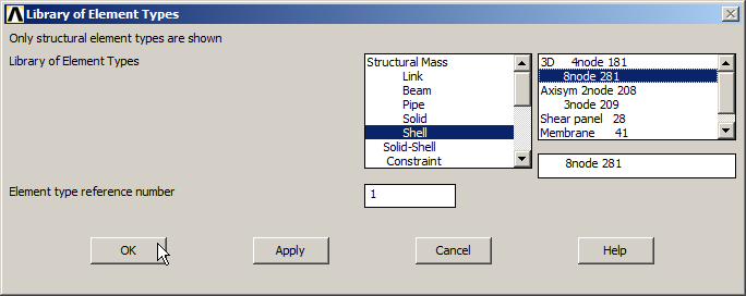
Figure 2. Element type: "Shell 8 node 281".
Now, input the mechanical properties of the aluminium (Figure 3):
Main Menu > Preprocessor > Material Props > Material Models
Define the material as "Structural – Linear – Elastic – Isotropic".
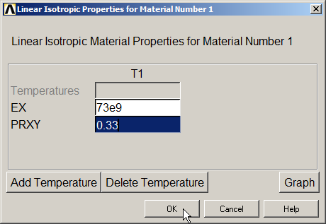
Figure 3. Material properties.
Now, input the value of the wall thickness:
Main Menu > Preprocessor > Sections > Shell > Lay-up
Figure 4 displays the window in which the value of the thickness is defined.
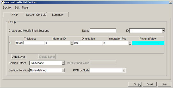
Figure 4. Thickness for "Shell" element.
Now, create a grid for the working plane from "WP Settings…".
Utility Menu > WorkPlane > WP Settings
The parameters for the grid are displayed in Figure 5.
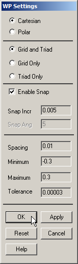
Figure 5. Parameters for the grid.
The grid can be displayed on the screen:
Utility Menu > WorkPlane > Display Working Plane
Now, create a circle located at (-0.06, 0) and radius 0.28 m, as indicated in Figure 6. This circle defines the curvature of the spherical caps.
Main Menu > Preprocessor > Modeling > Create > Lines > Arcs > Full Circle
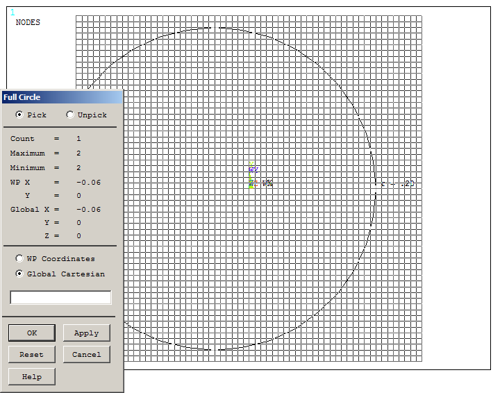
Figure 6. Creating a circle.
Figure 7 shows the graphic screen with the grid and the circle.
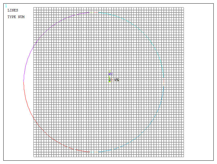
Figure 7. Graphic screen with the circle.
Next, create two keypoints that will define a straight line to divide the circle.
Main Menu > Preprocessor > Modeling > Create > Keypoints > On Working Plane
Create these two keypoints as indicated in Figure 8.
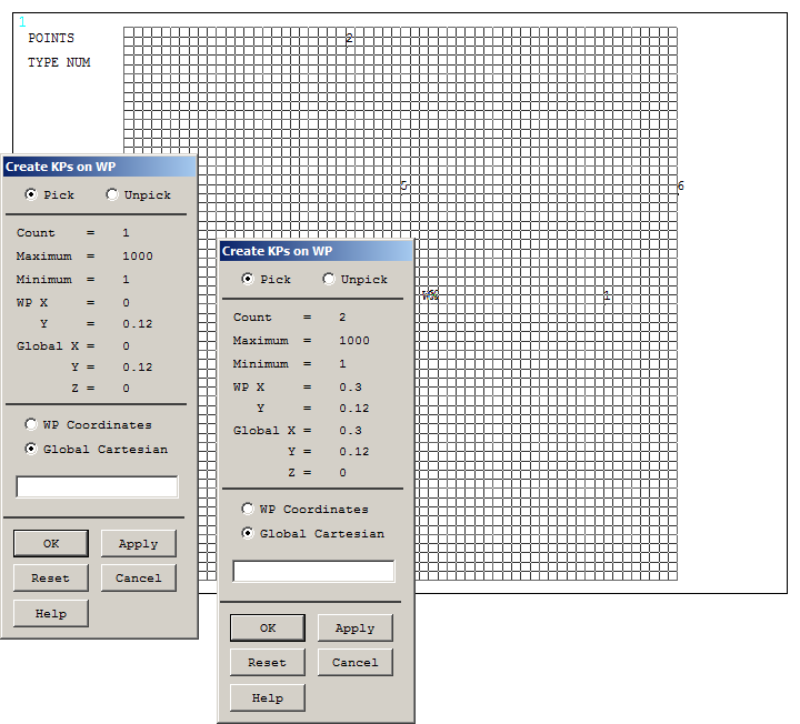
Figure 8. Creating two keypoints.
Now, create a straight line between the two keypoints:
Main Menu > Preprocessor > Modeling > Create > Lines > Lines > Straight Line
Figure 9 represents the created lines. Now, number the lines:
Utility Menu > PlotCtrls > Numbering
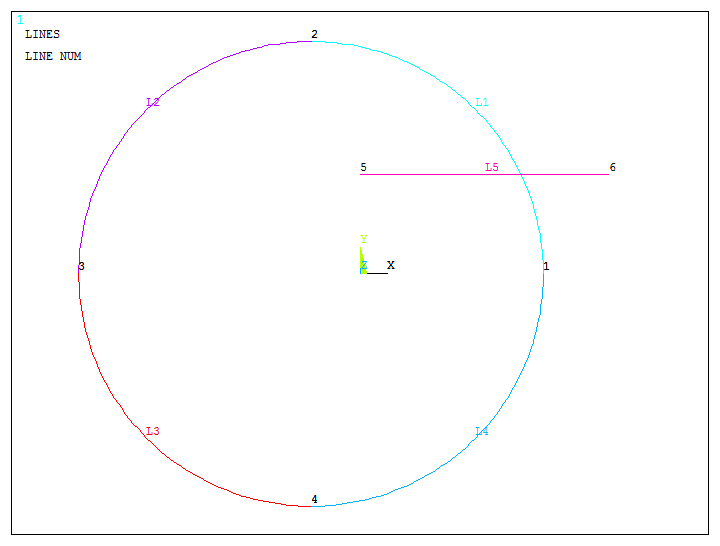
Figure 9. Created lines.
Now, divide one line of the circle in two different lines.
Main Menu > Preprocessor > Modeling > Operate > Booleans > Divide > Line by Line
First, select the circular line and "OK" (Figure 10).
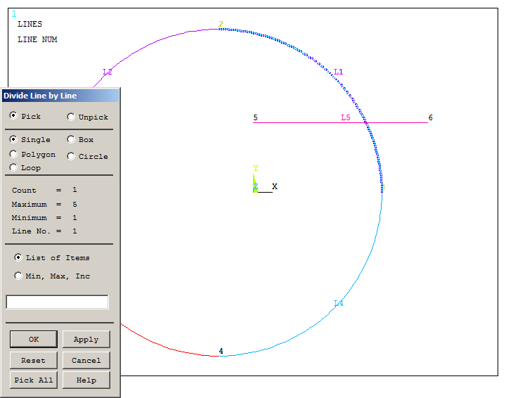
Figure 10. Selecting the circular line.
Next, select the straight line and "OK" (Figure 11).
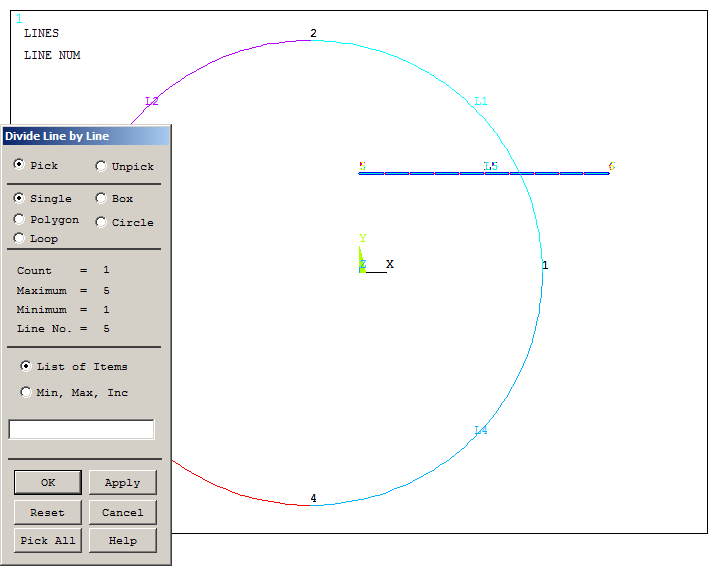
Figure 11. Selecting the straight line.
As displayed in Figure 12, a new line in the circle has been created.
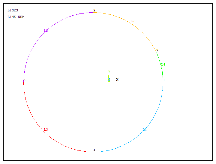
Figure 12. New line in the circle.
After that, delete the lines 2, 3, 4 and 7:
Main Menu > Preprocessor > Modeling > Delete > Line and Below
With the option "Lines and Below", all the geometric entities attached to these lines will be removed. Figure 13 shows the line 6 after deleting the other lines.
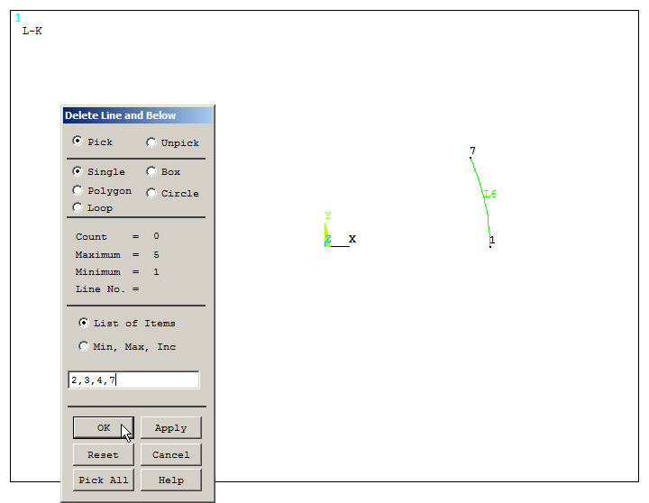
Figure 13. Deleting lines L2, L3, L4 and L7.
Now, copy line 6 with "Reflect Lines" operation:
Main Menu > Preprocessor > Modeling > Reflect > Lines
For this operation, define the parameters indicated in Figure 14.
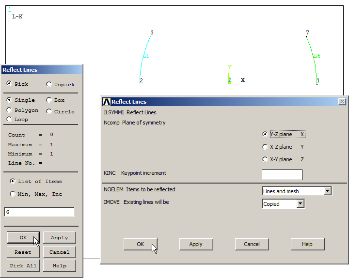
Figure 14. "Reflect Lines" operation.
Next, create a straight line between keypoints 3 and 6 (Figure 15):
Main Menu > Preprocessor > Modeling > Create > Lines > Lines > Straight Line.
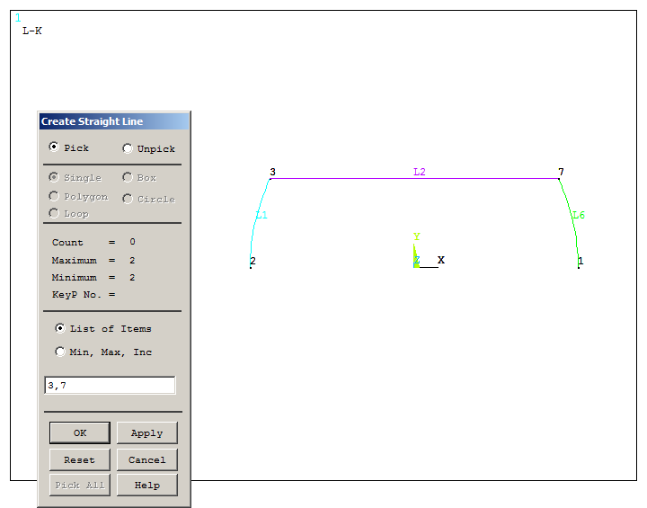
Figure 15. Line between keypoints 3 and 7.
Define the curvature by means of "Line Fillet" operation.
Main Menu > Preprocessor > Modeling > Create > Lines > Line Fillet
The first fillet radius is between lines L2 and L6, and the second one is between lines L1 and L2. The radius is 0.02 m, as indicated in Figure 16.
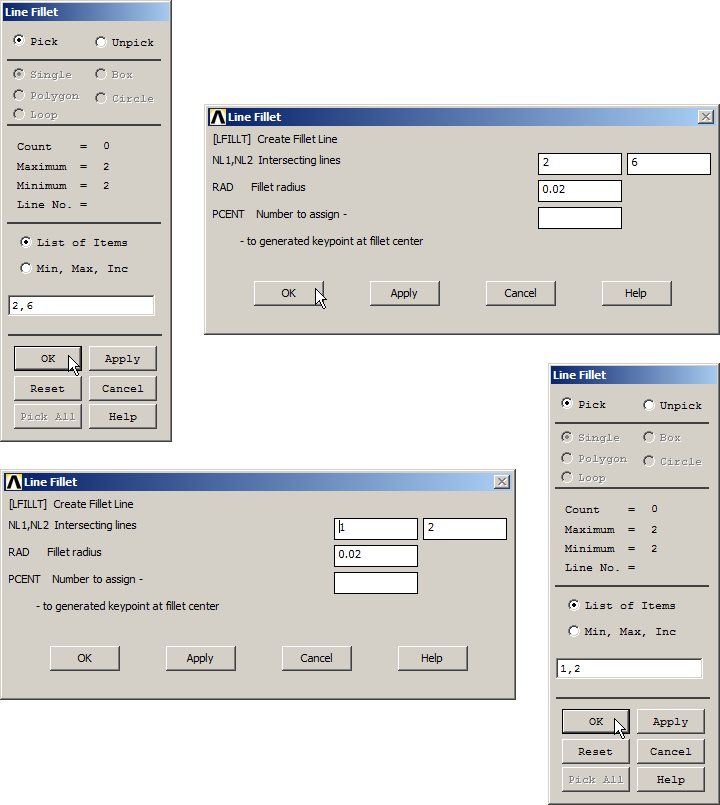
Figure 16. "Line Fillet" operation.
Figure 17 displays the lines after "Line Fillet" operation.
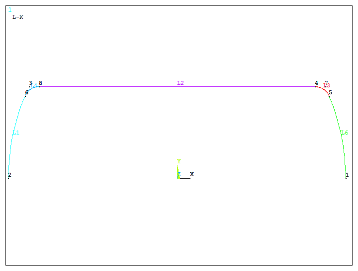
Figure 17. Lines after "Line Fillet" operation.
Finally, extrude these lines about axis.
Main Menu > Preprocessor > Modeling > Operate > Extrude > Lines > About Axis
Figure 18 indicates the process for extruding the lines. Select the lines, "OK", and then select the two keypoints that define the axis of symmetry. The revolution angle is 360º and there will be 4 areas.
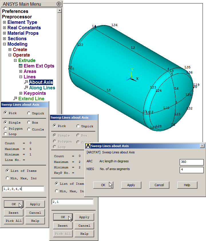
Figure 18. Pressure tank after "Extrude" operation.
When the geometry is completely defined, mesh the model. First, define the element size as 0.01 m (Figure 19).
Main Menu > Preprocessor > Meshing > Size Cntrls > ManualSize > Areas > All Areas
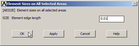
Figure 19. Element size.
Finish the meshing process. Figure 20 represents the meshed model of the pressure tank.
Main Menu > Preprocessor > Meshing > Mesh > Areas > Free
Click "Pick All".
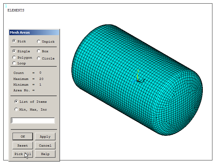
Figure 20. Meshed model.
LOADS AND BOUNDARY CONDITIONS
First of all, plot the lines of the model to apply the boundary conditions (Figure 21).
Utility Menu > Plot > Lines
Activate the option for numbering the keypoints from "Utility Menu – PlotCtrls – Numbering".
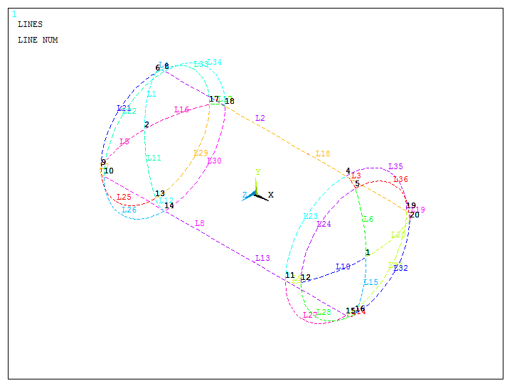
Figure 21. Lines of the model.
Restrict All Degrees of Freedom ("All DOF") at keypoint 2, as indicated in Figure 22.
Main Menu > Preprocessor > Loads > Define Loads > Apply > Structural > Displacement > On Keypoints
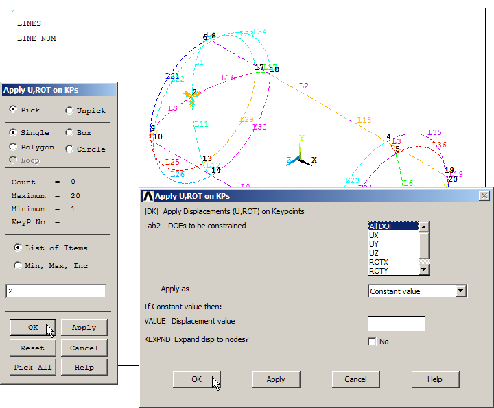
Figure 22. "All DOF" at keypoint 2.
After that, apply the pressure of 5 bar (500 000 Pa) to the walls of the pressure tank:
Main Menu > Preprocessor > Loads > Define Loads > Apply > Structural > Pressure > On Areas
And select "Pick All". Figure 23 represents the pressure tank with the applied pressure.
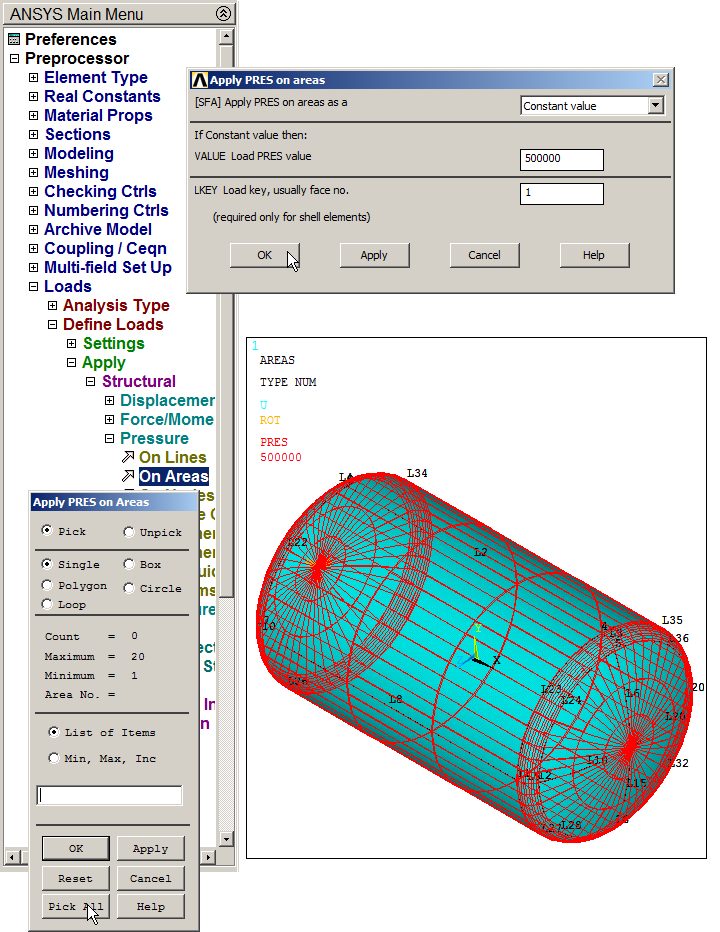
Figure 23. Pressure on areas.
The pressure can be displayed with "Arrows", as indicated in Figure 24.
Utility Menu > PlotCtrls > Symbols
And select "Arrows" in "Show pres and convect as" option.
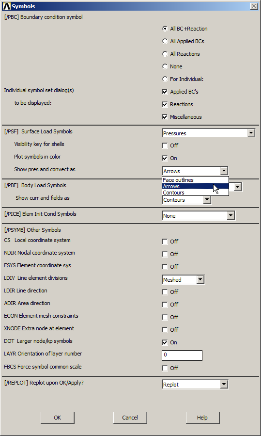
Figure 24. Selecting "Arrows" to represent the pressure.
Figure 25 represents the model with the applied pressure and boundary conditions.
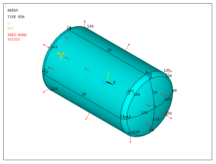
Figure 25. Pressure tank with load and boundary conditions.
SOLUTION
Solve the problem:
Main Menu > Solution > Solve > Current LS
"Solution is done!". Figure 26 shows the model after the calculation process.
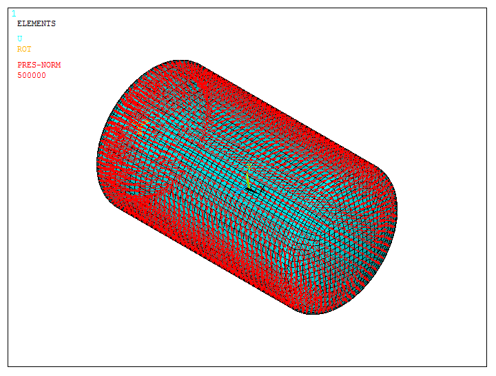
Figure 26. Solved model.
RESULTS
First of all, evaluate the deformation of the model:
Main Menu > General Postproc > Plot Results > Deformed Shape
And select "Def+undeformed" (Figure 27).
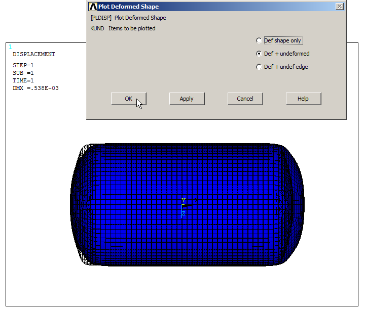
Figure 27. Deformed shape of the pressure tank.
Next, analyze the stress distribution in the pressure tank (Figure 28).
Main Menu > General Postproc > Plot Results > Contour Plot > Nodal Solu
And select "Stress – von Mises stress".
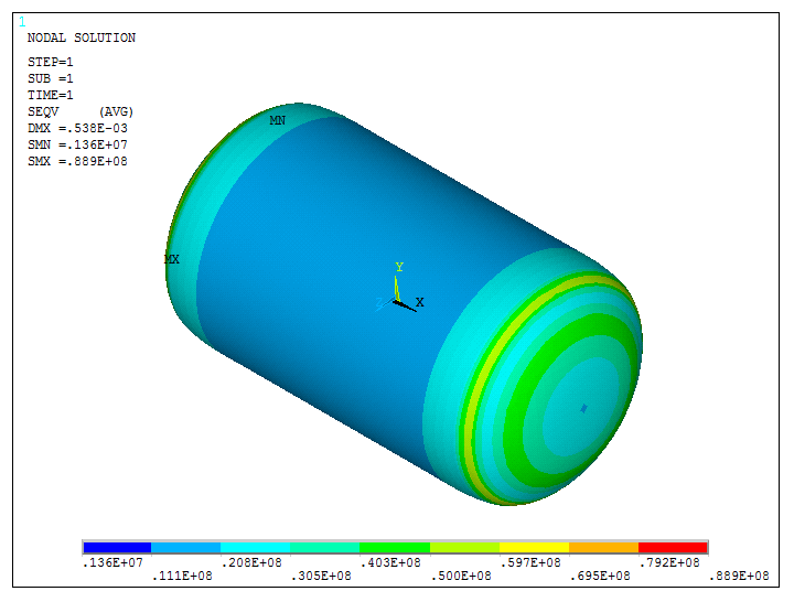
Figure 28. Stress distribution (von Mises stress).
It is observed that the maximum value of the stress is located at the spherical cap of the pressure tank. Analyze the stress distribution in this particular part of the model:
Utility Menu > Select Entities
Select "Areas – By Location", and define the range from 0 m to 0.3 m in X direction, as indicated in Figure 29.
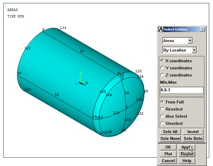
Figure 29. Selecting areas "By Location".
Then, from "Areas – By Num/Pick", click "Invert" as indicated in Figure 30. One of the spherical caps of the model is represented on the screen.
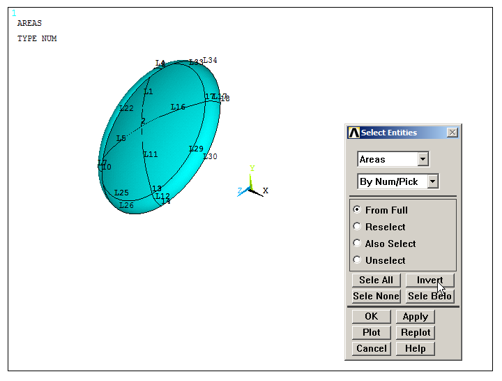
Figure 30. Selecting area by using "Invert".
After that, select "Elements – Attached to – Areas" and plot the stress distribution, as indicated in Figure 31.
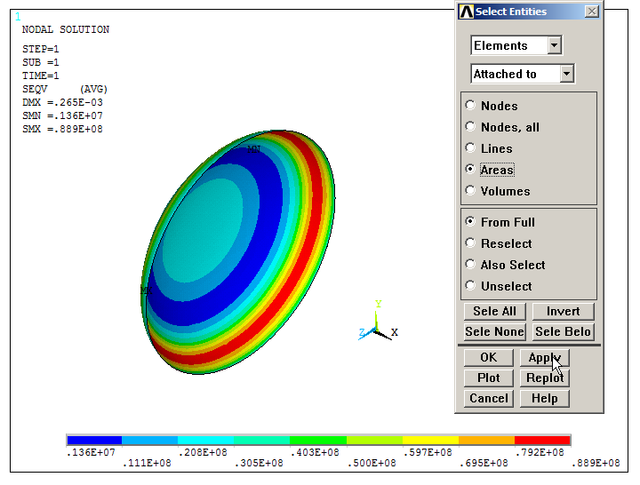
Figure 31. Stress distribution in the spherical cap of the pressure tank.
The maximum stress is located at the curvature.
Plot the model activating "ESHAPE" from "Size and Shape", as indicated in Figure 32.
Utility Menu > PlotCtrls > Style > Size and Shape
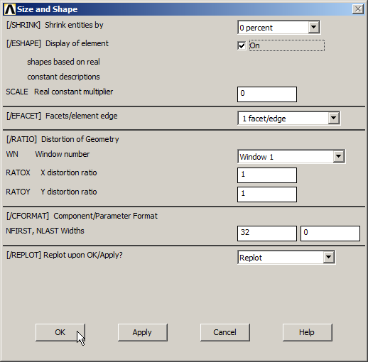
Figure 32. Representing the model with thickness.
A scaled model of the spherical cap is now represented in Figure 33. Because of that, it is observed that the results have changed.
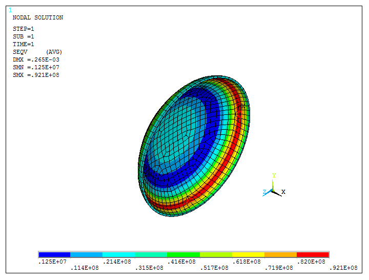
Figure 33. Stress distribution taking into account the thickness (scaled model).
Finally, animate the results (Figure 34).
Utility Menu > PlotCtrls > Animate > Deformed Results
Input the parameters that are displayed in the window "Animate Nodal Solution Data".
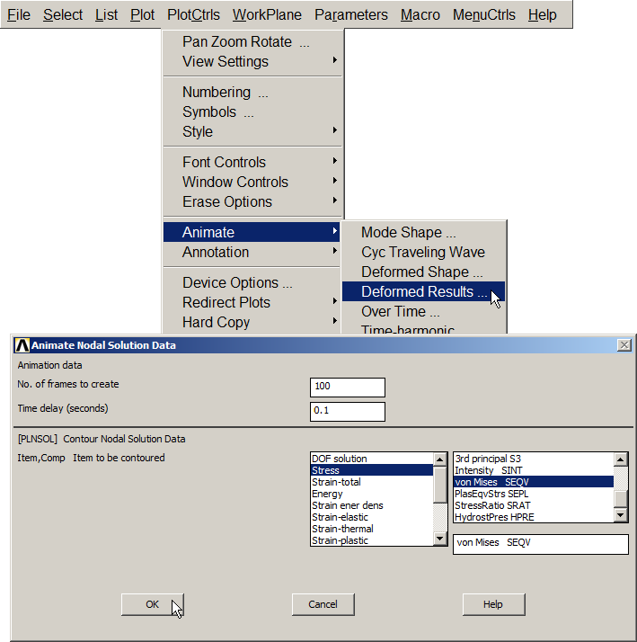
Figure 34. Animate results.
Activate the option "Forward Only" from the "Animation Controller" as indicated in Figure 35.
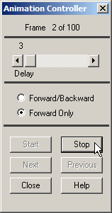
Figure 35. "Animation Controller" options.
The animated results can be saved as a video presentation (Figure 36):
Utility Menu > PlotCtrls > Animate > Save Animation
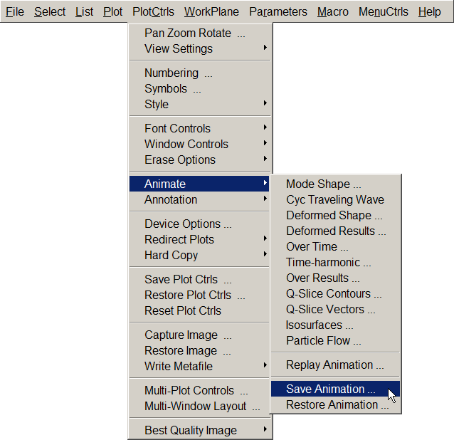
Figure 36. Save Animation.
Animation is saved as "anim" (*.avi) in the corresponding folder (Figure 37).
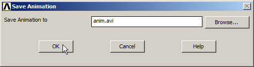
Figure 37. Save animation in the corresponding folder.
Figure 38 displays the animation of the results.
Figure 38. Video of the stress distribution in the model.