PROBLEM
Figure 1 represents the model of a pulley. Determine the stress distribution when a force of 5000 N is acting on the pulley due to the pressure of the transmission belt. The pulley is fixed in the central hole and the transmission belt covers 180º.
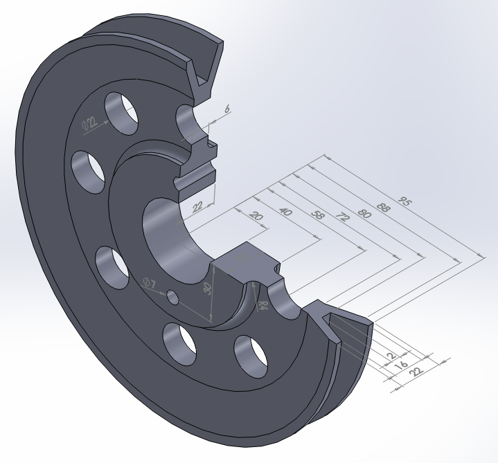
Figure 1. Pulley model.
Table 1 indicates the mechanical properties of the aluminium 6061 T6.
Table 1. Material properties.
| Aluminium 6061 T6 | |
| EAluminium | 69 GPa |
| νAluminium | 0.33 |
GEOMETRY OF THE MODEL
First of all, define the analysis type:
Main Menu > Preferences
Activate "Structural".
Now, change the jobname for this particular problem: "Pulley".
Utility Menu > File > Change Jobname
The element type for this problem is "SOLID 10 node 187" (Figure 2).
Main Menu > Preprocessor > Element Type > Add/Edit/Delete
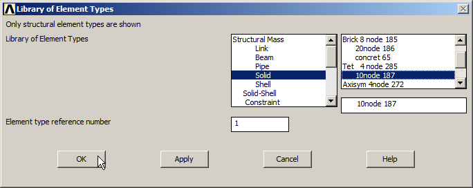
Figure 2. Element type: "SOLID 10 node 187".
Define the mechanical properties of the aluminium 6061 T6: modulus of elasticity (EX) and Poisson's ratio (PRXY), as indicated in Figure 3:
Main Menu > Preprocessor > Material Props > Material Models
The material is defined as "Structural – Linear – Elastic – Isotropic".
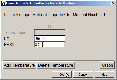
Figure 3. Material properties.
Create a grid for the working plane, as indicated in Figure 4.
Utility Menu > WorkPlane > WP Settings
The grid can be displayed on the screen with the option "Display Working Plane" from the "Utility Menu".
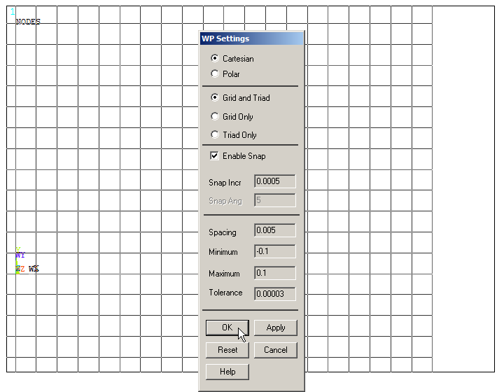
Figure 4. Grid for the working plane.
Now, create the keypoints indicated in Table 2.
Table 2. Keypoints coordinates.
| Keypoint | X (m) | Y (m) | Z (m) |
| 1 | 0.020 | 0.011 | 0 |
| 2 | 0.040 | 0.011 | 0 |
| 3 | 0.040 | 0.003 | 0 |
| 4 | 0.072 | 0.003 | 0 |
| 5 | 0.088 | 0.011 | 0 |
| 6 | 0.095 | 0.011 | 0 |
| 7 | 0.095 | 0.008 | 0 |
| 8 | 0.080 | 0.001 | 0 |
Main Menu > Preprocessor > Modeling > Create > Keypoints > In Active CS
Figure 5 displays the keypoints on the screen.
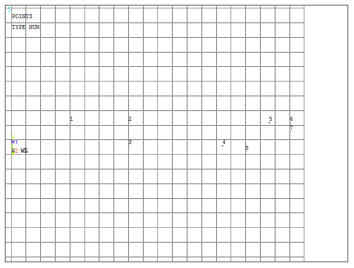
Figure 5. Created Keypoints.
After that, create the lines between the keypoints, as indicated in Figure 6.
Main Menu > Preprocessor > Modeling > Create > Lines > Lines > Straight Line
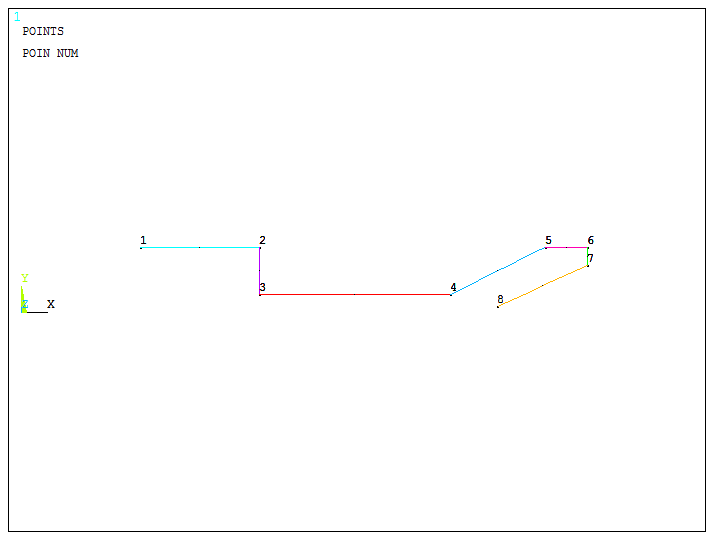
Figure 6. Straight lines between keypoints.
Number the keypoints (KP) and the lines (LINE):
Utility Menu > PlotCtrls > Numbering
Now, create a radius of curvature of 4 mm between lines L2 and L3, as indicated in Figure 7.
Main Menu > Preprocessor > Modeling > Create > Lines > Line Fillet
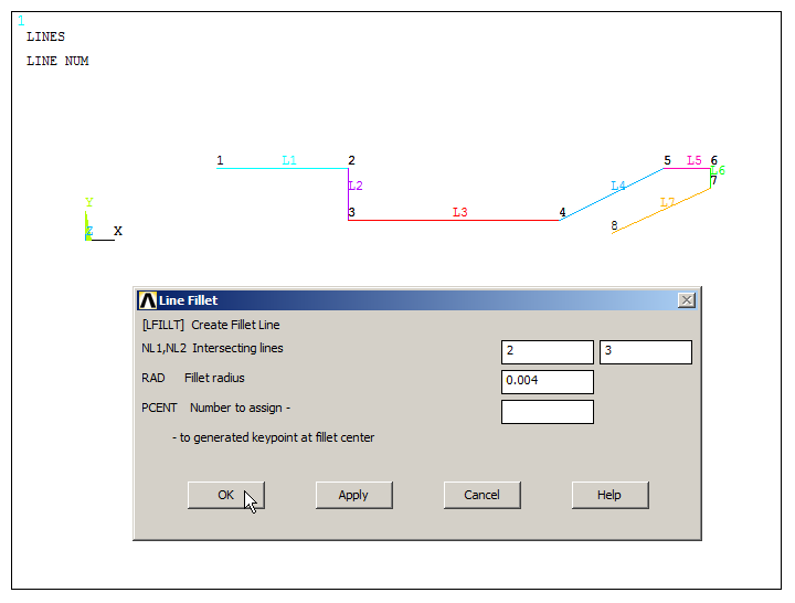
Figure 7. Radius of curvature between lines L2 and L3.
Copy the lines with the option "Reflect Lines".
Main Menu > Preprocessor > Modeling > Reflect > Lines
The parameters for this operation are indicated in Figure 8. Click "Pick All" and select "X-Z plane Y".
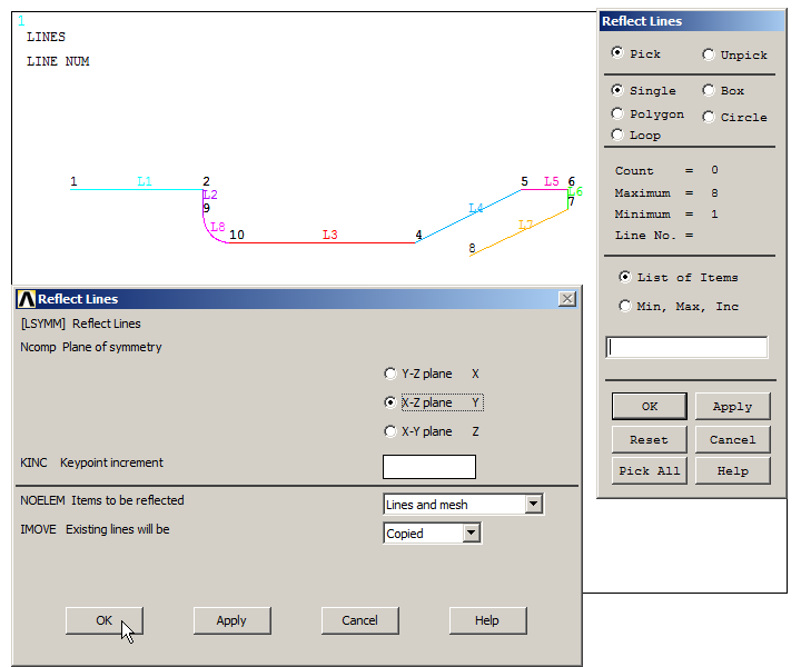
Figure 8. "Reflect Lines" operation.
Create the lines to close the polygon, as indicated in Figure 9.
Main Menu > Preprocessor > Modeling > Create > Lines > Lines > Straight Line
There are two new lines: the first one between keypoints 1 and 11, and the second one between keypoints 8 and 19.
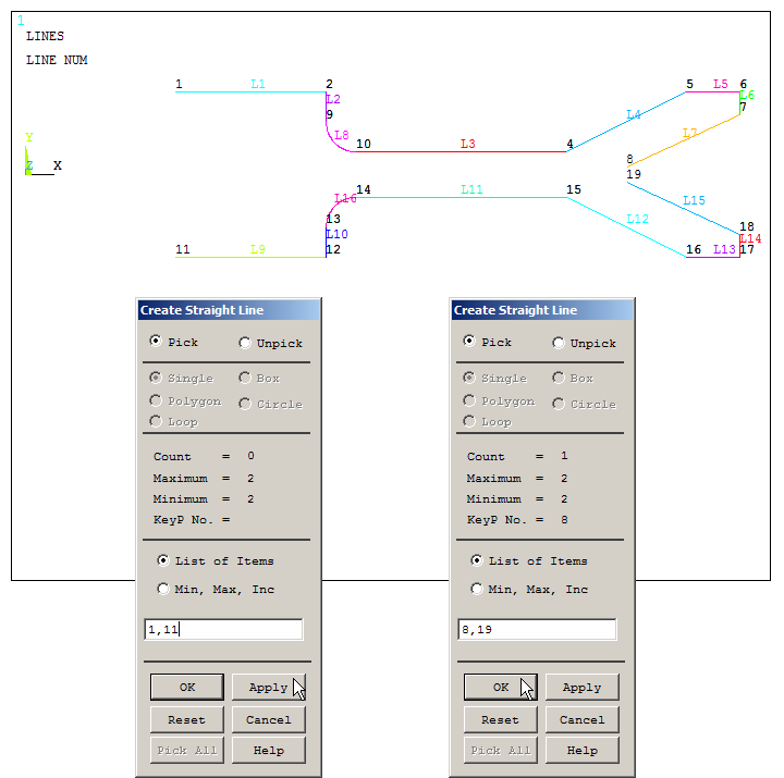
Figure 9. Create two lines to close the polygon.
Create the area as indicated in Figure 10.
Main Menu > Preprocessor > Modeling > Create > Areas > Arbitrary > By Lines
Select every line consecutively and "OK".
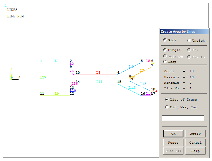
Figure 10. Create the area by lines.
To create the volume, an axis of revolution is required. For the axis, create two new keypoints. The coordinates of these keypoints are indicated in Figure 11.
Main Menu > Preprocessor > Modeling > Create > Keypoints > In Active CS
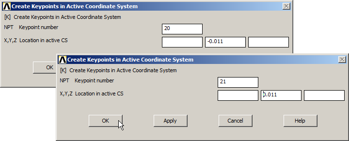
Figure 11. Create two keypoints for the axis of revolution.
Figure 12 displays the area and the keypoints 20 and 21.
Utility Menu > Plot > Multi-Plots
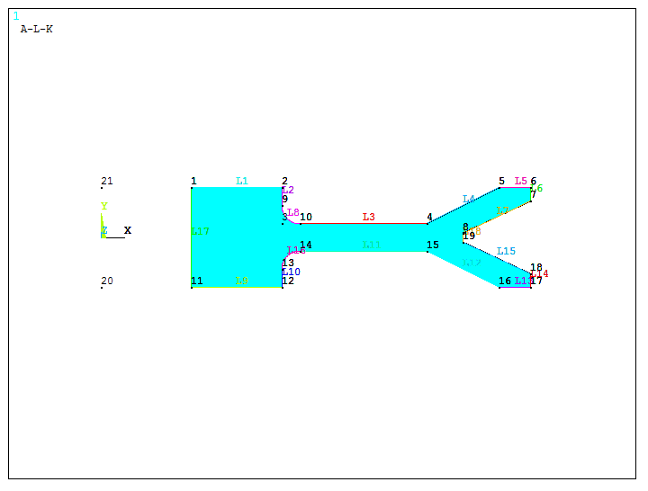
Figure 12. "Multi-Plots" option.
Extrude the area about the axis of revolution (360º).
Main Menu > Preprocessor > Modeling > Operate > Extrude > Areas > About Axis
First click on the area and then click on keypoints 20 and 21. Define four segments, as indicated in Figure 13.
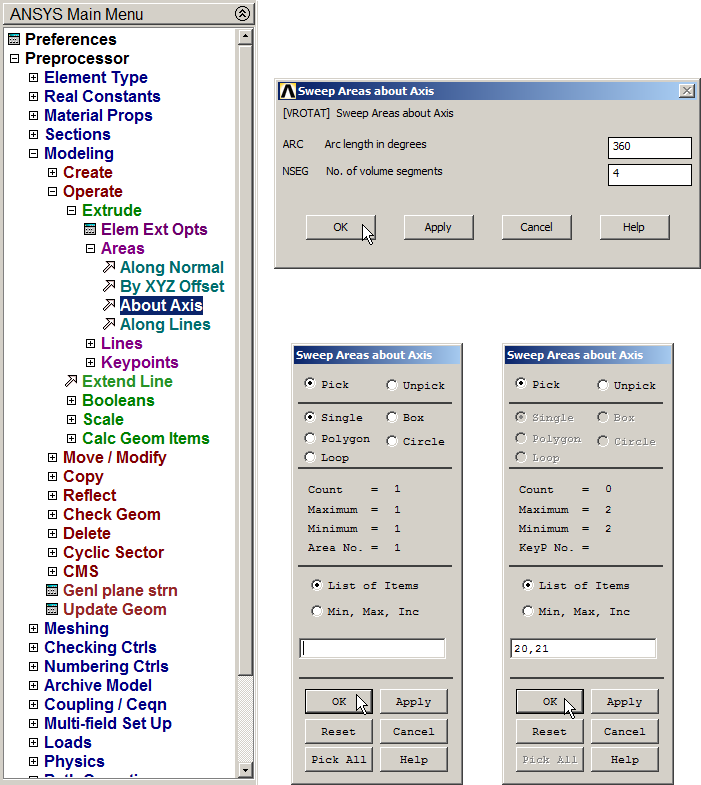
Figure 13. Extrude about axis.
Figure 14 displays the generated volume. Now, change the orientation of the working plane.
Utility Menu > WorkPlane > Offset WP by Increments
Rotate the working plane as indicated in Figure 14.
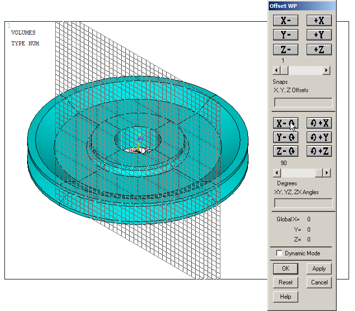
Figure 14. Pulley model and working plane.
Next, move the working plane 58 mm in the positive X direction and 11 mm in the negative Z direction (Figure 15).
Utility Menu > WorkPlane > Offset WP by Increments
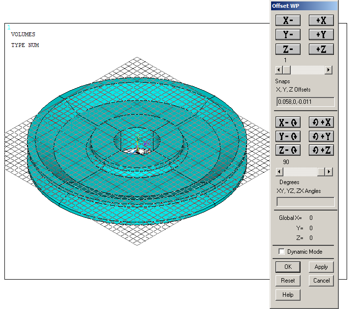
Figure 15. Moving the working plane.
Create a solid cylinder with the geometric characteristics indicated in Figure 16.
Main Menu > Preprocessor > Modeling > Create > Volumes > Cylinder > Solid Cylinder
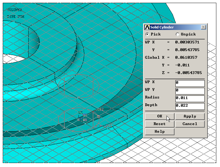
Figure 16. Create a solid cylinder.
This solid cylinder must be copied for every cylindrical hole. First, select angular units, as indicated in Figure 17.
Utility Menu > Parameters > Angular Units
And select "Degrees DEG".
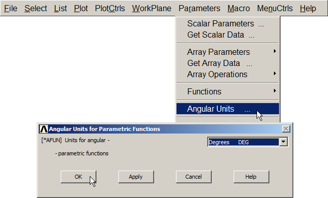
Figure 17. Select "Degrees DEG".
After that, change the coordinate system (Figure 18).
Utility Menu > WorkPlane > Change Active CS to > Global Cylindrical Y
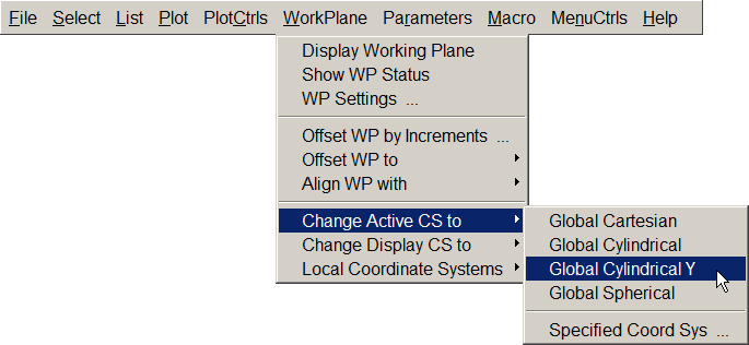
Figure 18. Change the coordinate system.
Then copy the solid cylinder eight times (the original is included in the number of copies).
Main Menu > Preprocessor > Modeling > Copy > Volumes
Click on the solid cylinder and input the parameters indicated in Figure 19.
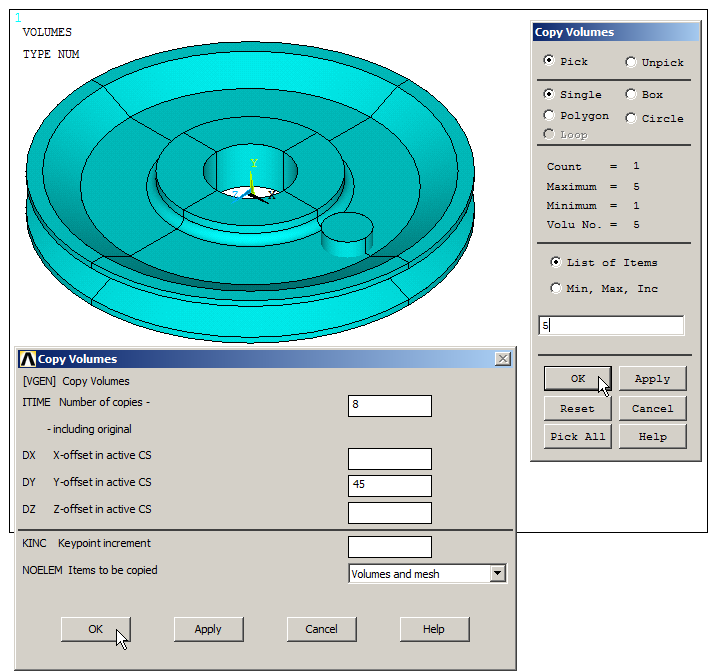
Figure 19. "Copy Volumes" operation.
Again, change the coordinate system (Figure 20).
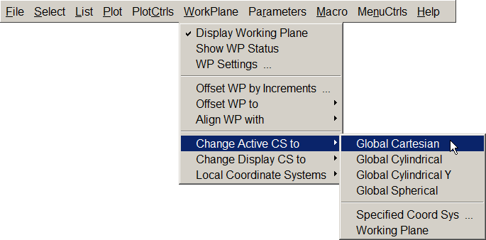
Figure 20. Cartesian coordinate system.
Now, subtract the cylindrical volumes to generate the holes.
Main Menu > Preprocessor > Modeling > Operate > Booleans > Subtract > Volumes
First select the global volume (four parts), "OK" and then the eight cylinders and "OK" (Figure 21).
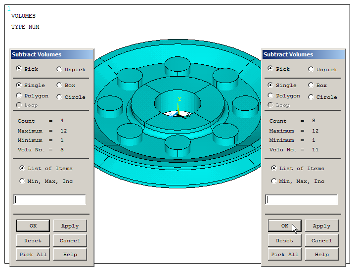
Figure 21. Subtract the cylindrical volumes.
To complete the model, there are two cylindrical holes located at the central part. Move the working plane at keypoint 20.
Utility Menu > WorkPlane > Offset WP to > Keypoints
And select the keypoint 20 (Figure 22).
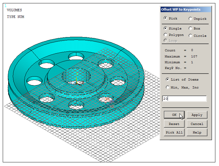
Figure 22. Move the working plane at keypoint 20.
Now, create a cylindrical volume as indicated in Figure 23.
Main Menu > Preprocessor > Modeling > Create > Volumes > Cylinder > Solid Cylinder
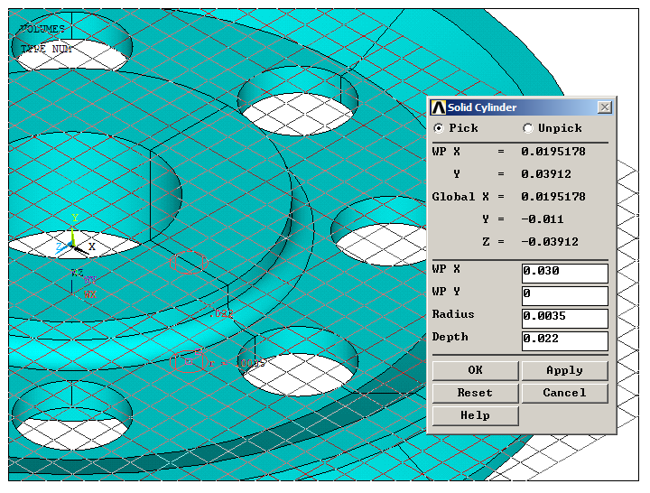
Figure 23. Create a new solid cylinder.
Copy this volume.
Main Menu > Preprocessor > Modeling > Reflect > Volumes
Input the parameters indicated in Figure 24.
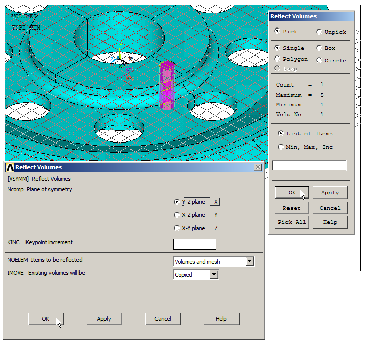
Figure 24. "Reflect Volumes" to copy the solid cylinder.
Repeat the "Subtract" operation with these two cylindrical volumes (Figure 25).
Main Menu > Preprocessor > Modeling > Operate > Booleans > Subtract > Volumes
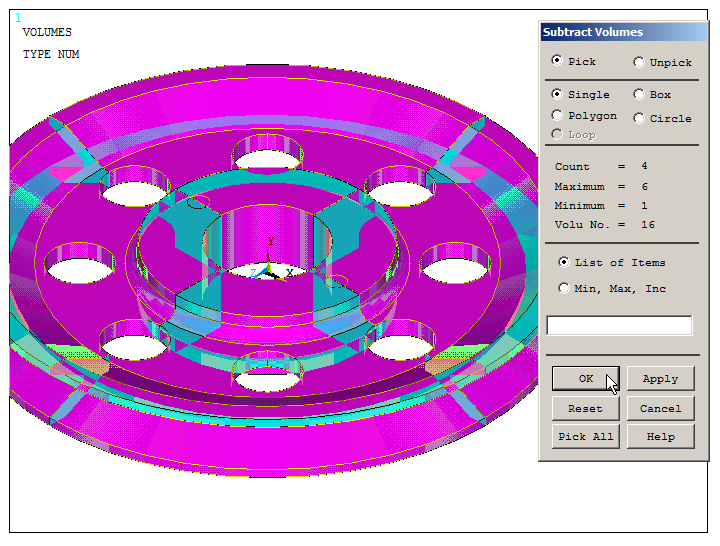
Figure 25. "Subtract Volumes" operation.
Figure 26 displays the "Subtract Volumes" operation for these two cylindrical volumes.
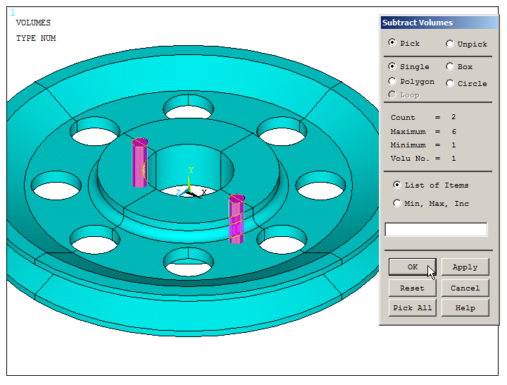
Figure 26. Subtract the two solid cylinders at the central part.
The next step is to mesh the model. The element size is 4 mm as indicated in Figure 27.
Main Menu > Preprocessor > Meshing > Size Cntrls > ManualSize > Global > Size
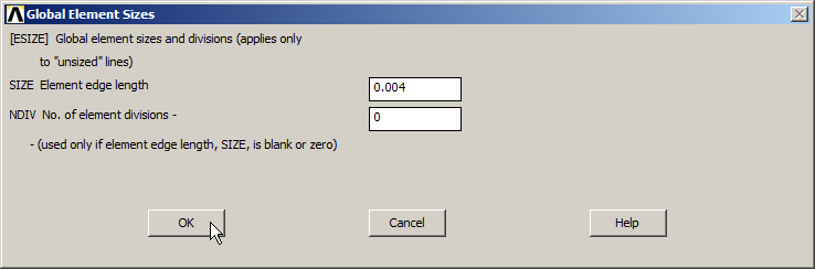
Figure 27. Define the element size.
Finish the meshing process.
Main Menu > Preprocessor > Meshing > Mesh > Volumes > Free
Click "Pick All" (Figure 28).
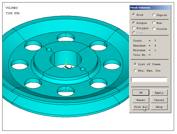
Figure 28. "Mesh Volumes" operation.
LOADS AND BOUNDARY CONDITIONS
The pulley is fixed at the central hole, so restrict all degrees of freedom (All DOF) on this area.
Main Menu > Preprocessor > Loads > Define Loads > Apply > Structural > Displacement > On Areas
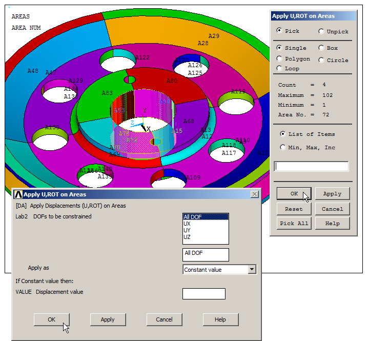
Figure 29. "All DOF" at the central hole.
For the load, the transmission belt produces a pressure on the pulley groove, as displayed in Figure 30. As a first approach, the value of the pressure is 1000000 Pa.
Main Menu > Preprocessor > Loads > Define Loads > Apply > Structural > Pressure > On Areas
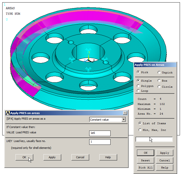
Figure 30. Apply pressure on areas.
Figure 31 displays the model with the pressure and the boundary conditions.
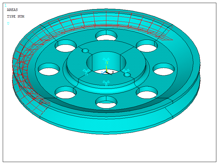
Figure 31. Model with the pressure and the boundary conditions.
SOLUTION
Solve the problem.
Main Menu > Solution > Solve > Current LS
"Solution is done!".
Figure 32 displays the model after the solution process.
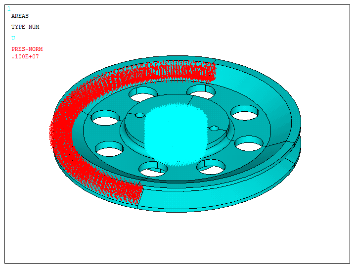
Figure 32. Pulley model after solution.
First of all, evaluate the value of the reaction forces.
Main Menu > General Postproc > List Results > Reaction Solu
Select "All items".
The values are listed in Figure 33.
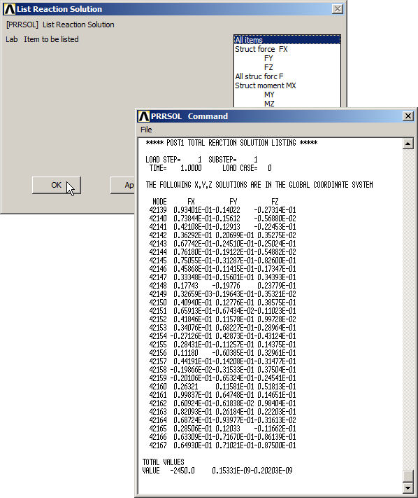
Figure 33. List Results.
It is observed that the total value is 2450 N.
Since the applied force of 5000 N is tangent at two particular points, input a new value of the pressure to obtain a total reaction force of 10000 N.
Main Menu > Solution > Loads > Define Loads > Delete > Structural > Pressure > On Areas
Click "Pick All".
As described before, apply the new value of the pressure (Figure 34).
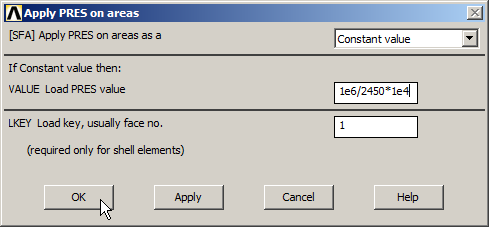
Figure 34. New value of the pressure.
Again, solve the problem (Figure 35).
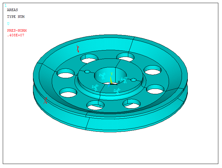
Figure 35. Solve the problem.
The results are listed in Figure 36. Now, it is observed that the reaction force is 10000 N.
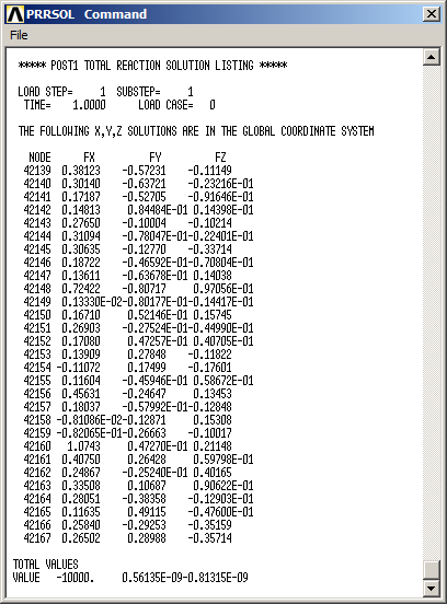
Figure 36. List results.
RESULTS
Evaluate the stress distribution in the pulley (Figure 37).
Main Menu > General Postproc > Plot Results > Contour Plot > Nodal Solu
And select "von Mises stress".
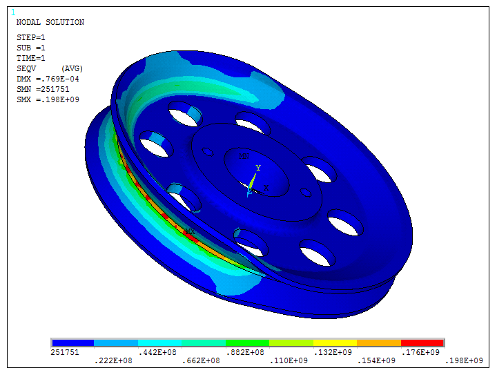
Figure 37. Stress distribution in the pulley.
Now, define the minimum and maximum contour values for the stress.
Utility Menu > PlotCtrls > Style > Contours > Uniform Contours
Input the parameters indicated in Figure 38.
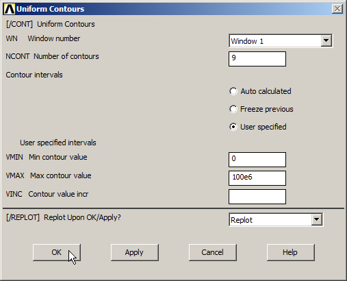
Figure 38. Limit the contour values for the stress.
Now, Figure 39 displays the stress distribution in the model. The parts of the model that exceed the limits, are represented in grey colour.
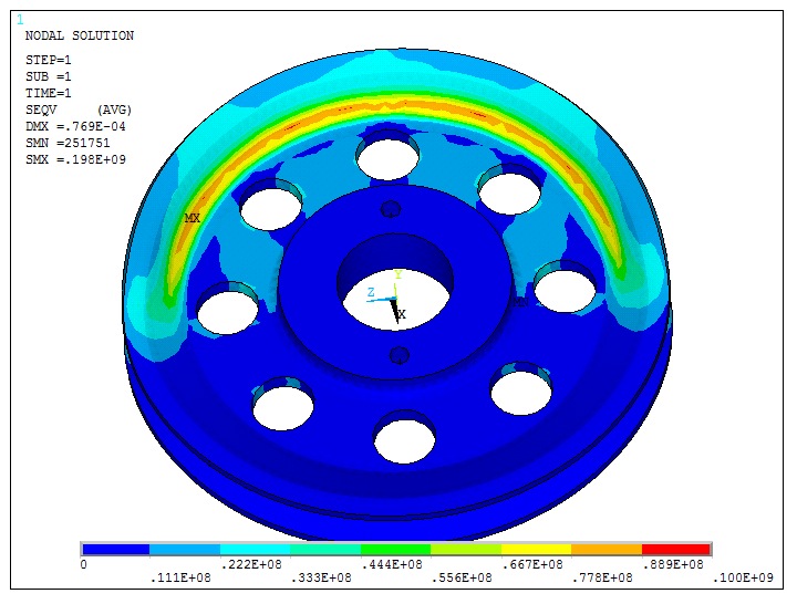
Figure 39. Stress distribution with the contour values.
Finally, display the part of the model in which the stress distribution is significant (Figure 40).
Utility Menu > Select > Entities
Select the two volumes and then select the elements attached to those volumes.
Utility Menu > Plot > Volumes
The results are displayed in Figure 40.
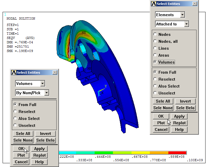
Figure 40. Stress distribution in a particular part of the model.