PROBLEM
Figure 1a represents a picture of a bridge that is made with two planar trusses. Figure 1b shows the scheme of one planar truss.
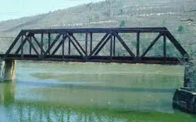
Figure 1a. Planar truss.
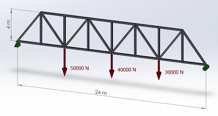
Figure 1b. Truss model.
Determine:
Tables 1 and 2 indicate the required data to solve this particular problem.
Table 1. Material properties.
| Steel | |
| Esteel | 210 GPa |
| Sy steel | 275 MPa |
| νsteel | 0.3 |
Table 2. Cross section of the bars.
| Section | 40 cm2 |
GEOMETRY OF THE MODEL
First of all, a new name is defined for this particular problem. In this case the name "Planar truss" (Figure 2).
Utility Menu > File > Change Title
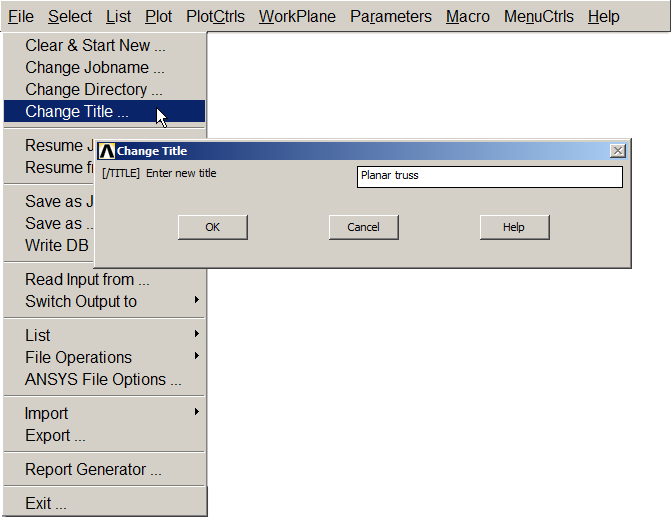
Figure 2. "Planar truss".
From "Preferences" it is defined the type of analysis, that is structural (Figure 3).
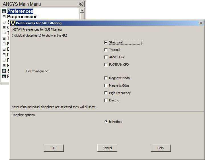
Figure 3. Structural analysis.
To solve this particular problem, LINK 180 element is selected (Figure 4):
Main Menu > Preprocessor > Element Type > Add/Edit/Delete
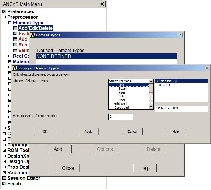
Figure 4. LINK 180 element.
The cross sectional area is the real constant (Figure 5):
Main Menu > Preprocessor > Real Constants > Add/Edit/Delete
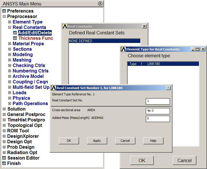
Figure 5. Real Constants.
Then, we have to define the mechanical properties of the material, that is the modulus of elasticity (EX) and the Poisson's ratio (PRXY) (Figure 6):
Main Menu > Preprocessor > Material Props > Material Models
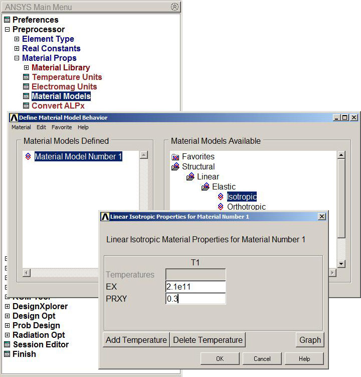
Figure 6. Mechanical properties of the material.
After that, we start by introducing the coordinates of the keypoints, that are the joints of the members (Figure 7):
Main Menu > Preprocessor > Modeling > Create > Keypoints > In Active CS
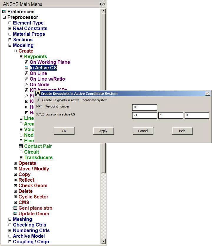
Figure 7. Create coordinates.
Table 3 shows the coordinates of the keypoints (meters):
Table 3. Keypoint coordinates.
| KEYPOINT | X | Y |
| 1 | 0 | 0 |
| 2 | 3 | 0 |
| 3 | 6 | 0 |
| 4 | 9 | 0 |
| 5 | 12 | 0 |
| 6 | 15 | 0 |
| 7 | 18 | 0 |
| 8 | 21 | 0 |
| 9 | 24 | 0 |
| 10 | 3 | 4 |
| 11 | 6 | 4 |
| 12 | 9 | 4 |
| 13 | 12 | 4 |
| 14 | 15 | 4 |
| 15 | 18 | 4 |
| 16 | 21 | 4 |
The graphic screen with the 16 keypoints is represented in Figure 8.
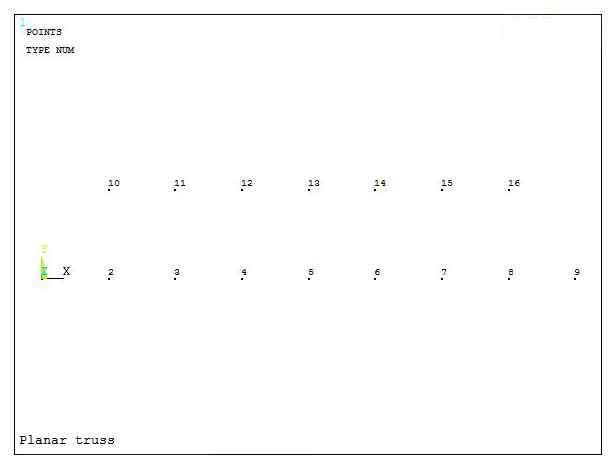
Figure 8. Keypoints of the truss.
Next, the bars connected at keypoints have to be created by lines (Figure 9):
Main Menu > Preprocessor > Modeling > Create > Lines > Straight Line
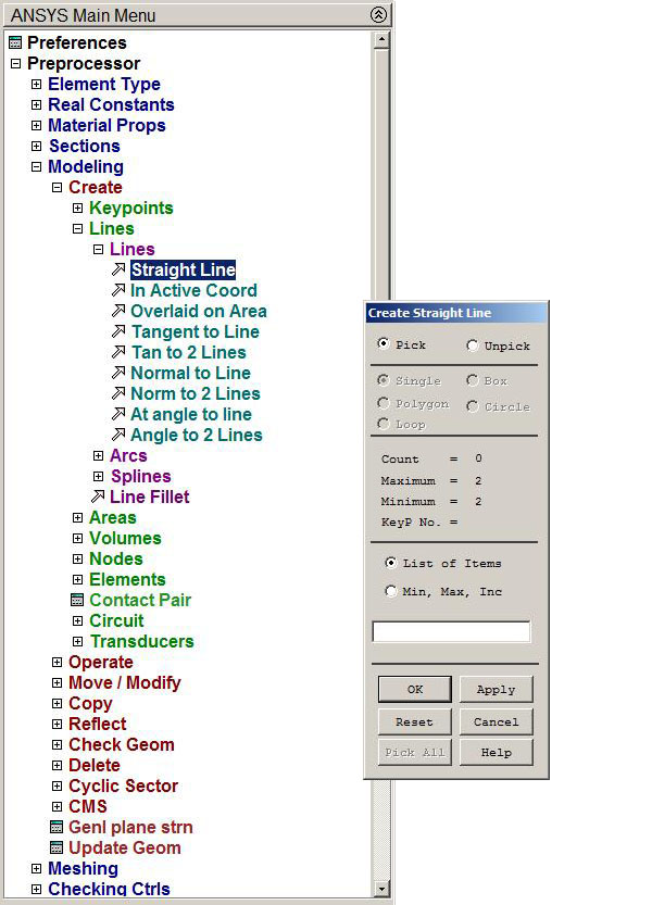
Figure 9. Defining lines.
Figure 10 is the model of the planar truss.
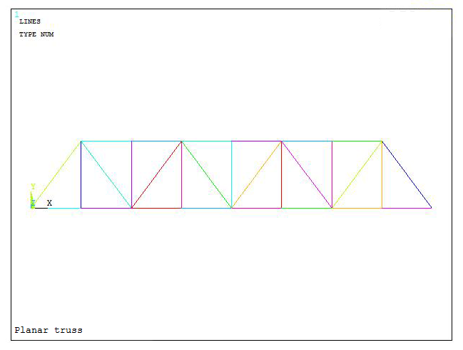
Figure 10. Model of the planar truss.
Then, the lines have to be meshed:
Main Menu > Preprocessor > Meshing > Size Cntrls > Manual Size > Lines > All Lines
Since these bars are two-force members that have axial stress, only one division per member is needed (NDIV No. of element divisions), as indicated in Figure 11.
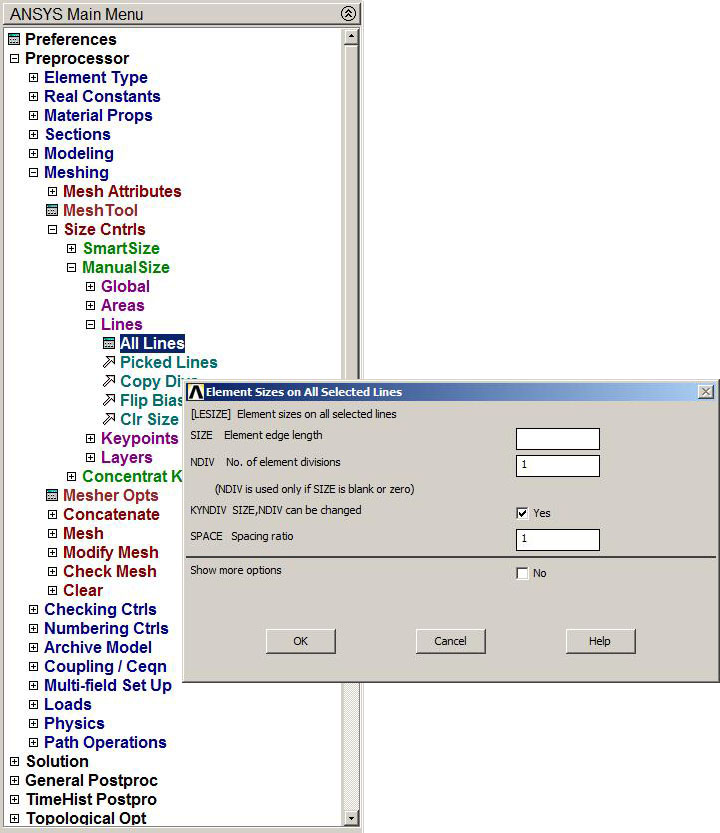
Figure 11. Element sizes for the members.
Figure 12 represents the meshed planar truss.
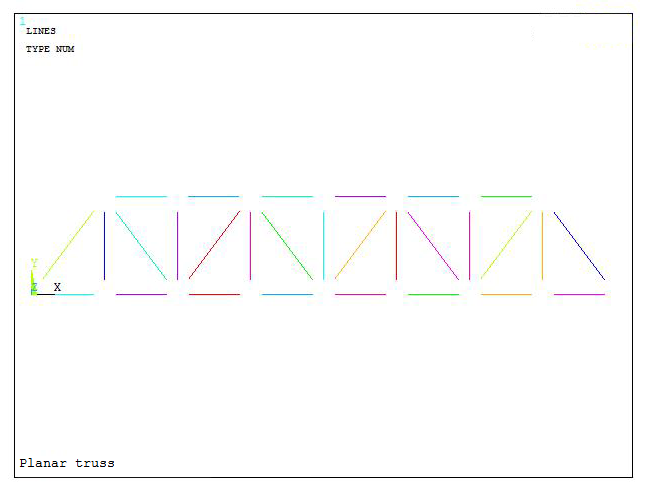
Figure 12. Meshed planar truss.
To finish the mesh process (Figure 13):
Main Menu > Preprocessor > Meshing > Mesh > Lines
And select "Pick All".
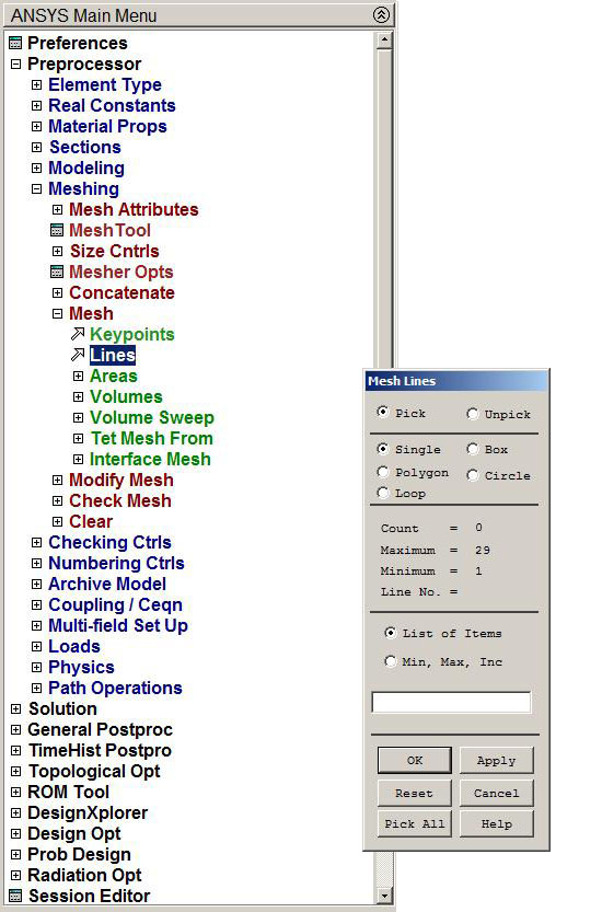
Figure 13. Mesh Lines.
Figure 14 represents the model of the planar truss, once it has been meshed.
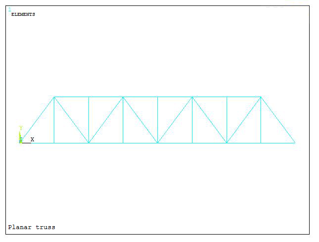
Figure 14. Model of the meshed planar truss.
LOADS AND BOUNDARY CONDITIONS
The next stage is to define the boundary conditions and the loads. First of all, we define the restrictions on the supports:
Main Menu > Preprocessor > Loads > Define Loads > Apply > Structural > Displacement > On Keypoints
On the left support, we select "ALL DOF" to restrict all degrees of freedom. In a planar model that is to restrict displacements in UX, UY and UZ directions (Figure 15).
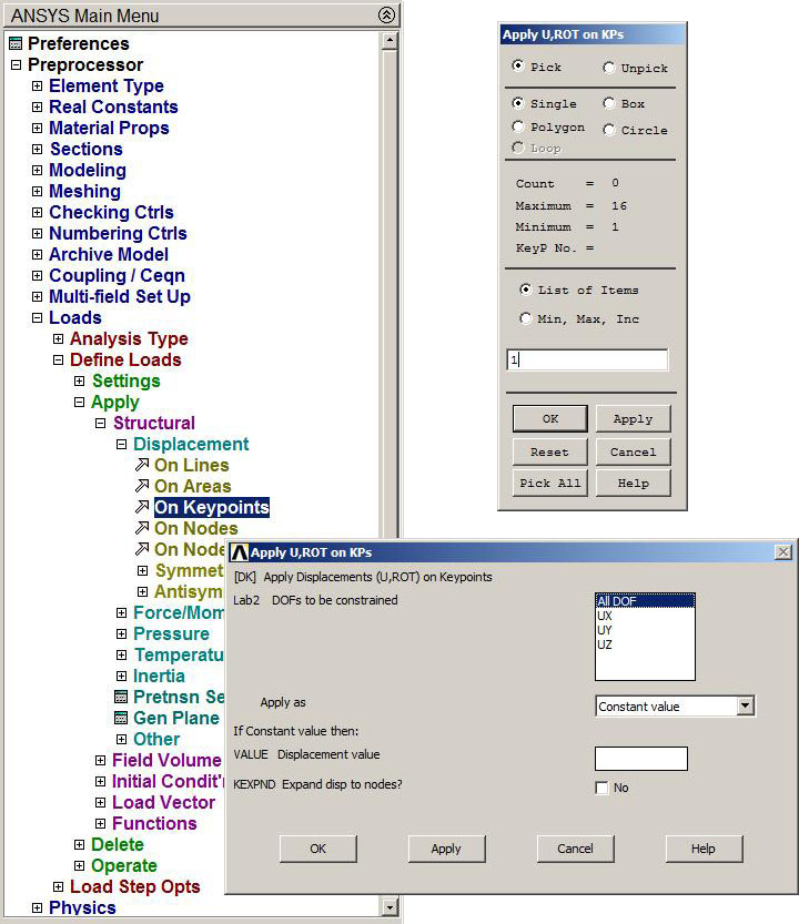
Figure 15. ALL DOF for the left support.
In the same way, the right support is restricted, but only UY and UZ displacements (Figure 16):
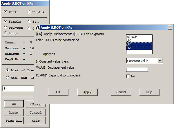
Figure 16. UY and UZ for the right support.
Figure 17 represents the model with the support conditions.
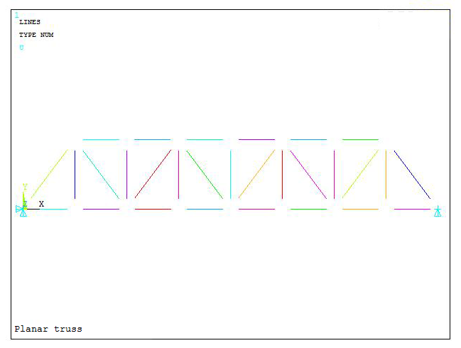
Figure 17. Model with support conditions.
After the definition of the support conditions, we have to define the loads acting on the truss:
Main Menu > Preprocessor > Loads > Define Loads > Apply > Structural > Force/Moment > On Keypoints
Figures 18, 19 and 20 show the application of the three loads in the negative direction UY.
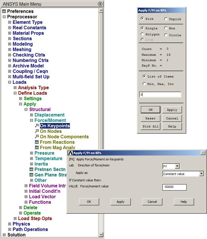
Figure 18. Application of the 50 kN load.
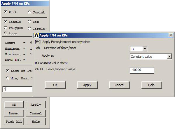
Figure 19. Application of the 40 kN load.
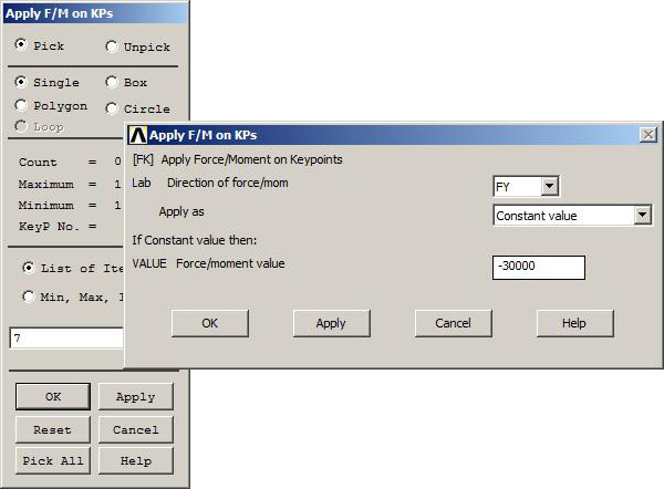
Figure 20. Application of the 30 kN load.
Figure 21 is the graphic screen with the finished model, that is with geometry, support conditions and loads.
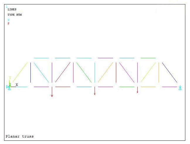
Figure 21. Finished model.
SOLUTION
Once the model is defined, we have to solve the structure:
Main Menu > Solution > Solve > Current LS
"Solution is done!" message appears in Figure 22.
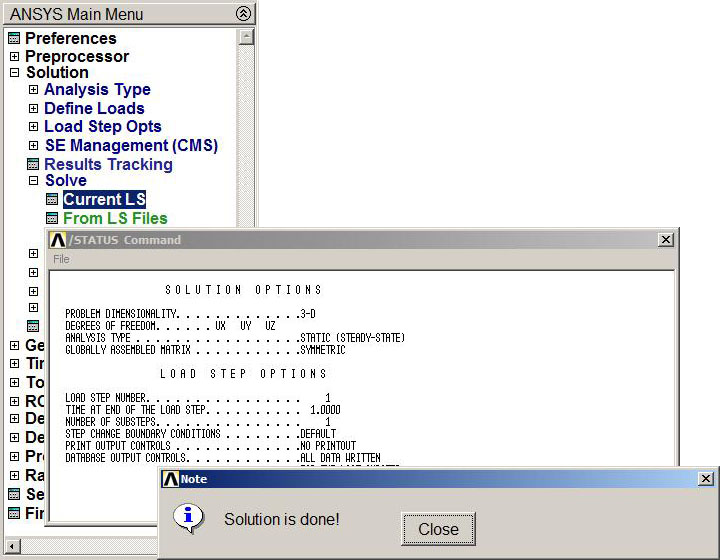
Figure 22. Solution is done.
RESULTS
Finally, the results have to be analyzed. First of all, the deformation of the planar truss from "General Postprocessor" (Figure 23):
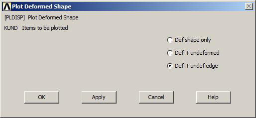
Figure 23. Plot Deformed Shape.
Figure 24 represents the deformation of the truss with the value for the maximum deformation (DMX).
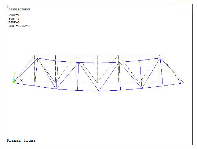
Figure 24. Deformation of the truss.
To evaluate the stress distribution, it is necessary to define a table:
Main Menu > General Postproc > Element Table > Define Table
For stresses we define a label (Figure 25): AXIALSTR. Select "By sequence num", "LS", "1" (consult ANSYS help).

Figure 25. Define a label for stresses.
The generated table is represented in Figure 26.
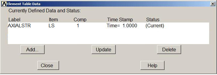
Figure 26. Element Table Data.
Now, the stress distribution is plotted (Figure 27):
Main Menu > General Postproc > Element Table > Plot Elem Table

Figure 27. Plot Element Table.
The graphic screen with the stress distribution in the truss is represented in Figure 28. The maximum value is SMX.
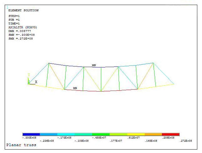
Figure 28. Stress distribution in the truss.
Sometimes it is useful to number the elements in order to evaluate the results in a more detailed way (Figure 29):
Utility Menu > PlotCtrls > Numbering
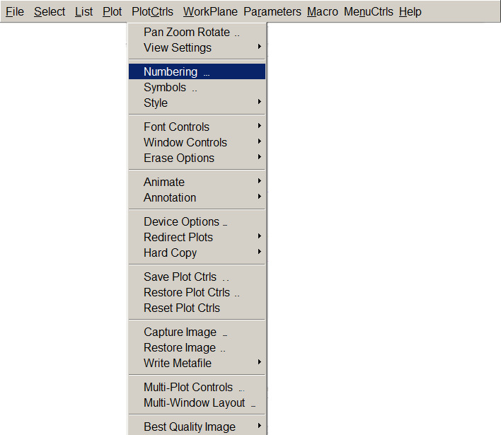
Figure 29. Numbering elements.
Click on "Element numbers" (Figure 30):
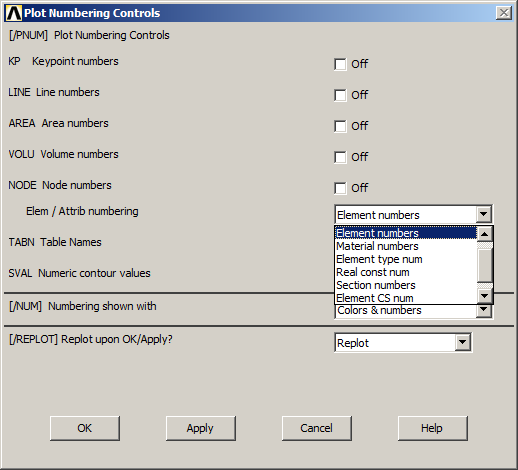
Figure 30. Plot Numbering Controls.
The result of numbering the elements is represented in Figure 31.
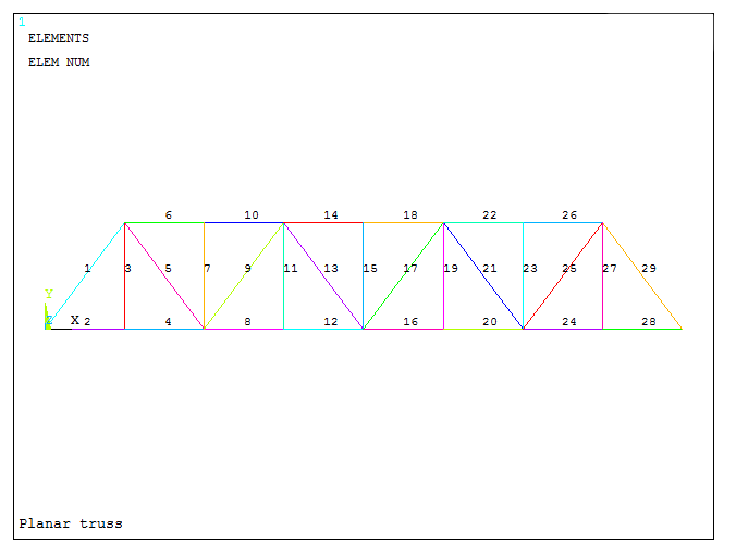
Figure 31. Truss with numbered elements.
Then we can list these results (Figure 32):
Main Menu > General Postproc > Element Table > List Elem Table
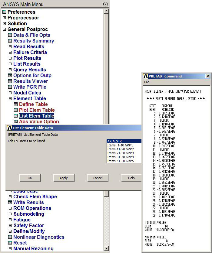
Figure 32. List Element Table.
The other result of interest is the value of the external reactions (Figure 33):
Main Menu > General Postproc > List Results > Reaction Solu
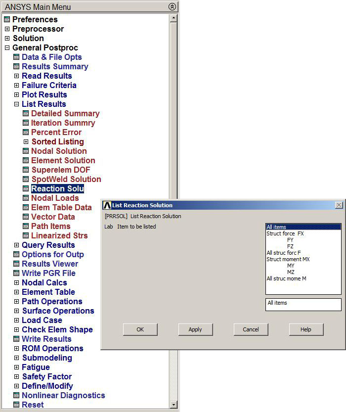
Figure 33. List Reaction Solution.
Figure 34 shows the list of the external reactions at nodes 1 and 9.
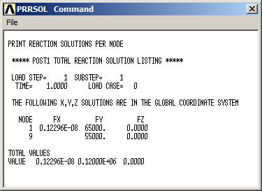
Figure 34. External reactions at nodes 1 and 9.
To represent all the results in one single graphic screen, we have to select the following option (Figure 35):
Utility Menu > PlotCtrls > Symbols
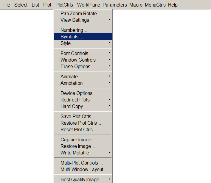
Figure 35. "Symbols" option.
Then, select "For Individual" option (Figure 36).
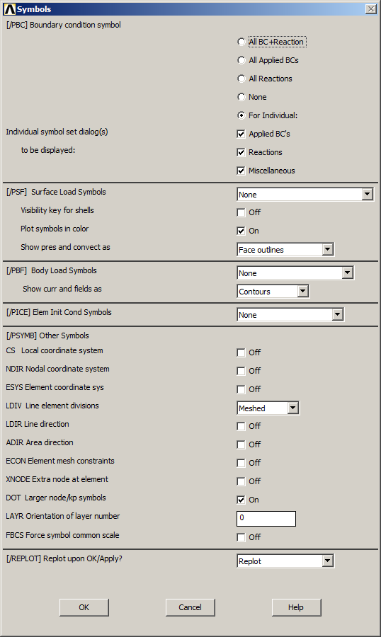
Figure 36. Select "For Individual".
Figures 37 and 38 represent the windows in which we have to select "Symbol" in "Applied translations" and "Symbol+Value" in "Applied forces" and in "Postproc reaction force". After that, click on "OK"..
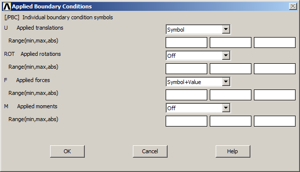
Figure 37. "Symbol" in "Applied translations" and "Symbol+Value" in "Applied forces".
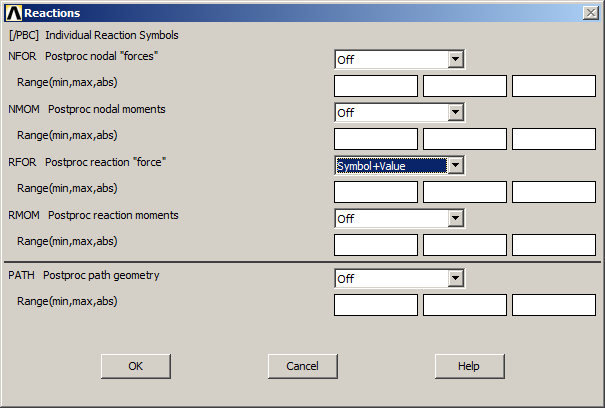
Figure 38. "Symbol+Value" in "Postproc reaction force".
On the other hand, unselect "Miscellaneous Boundary Conditions".
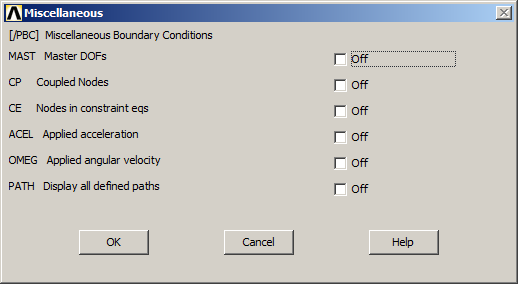
Figure 39. Unselect "Miscellaneous Boundary Conditions".
Once these options have been defined, Figures 40 and 41 represent the results.

Figure 40. Def + undef edge.
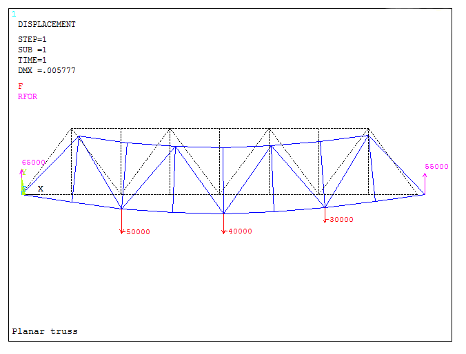
Figure 41. Graphic screen with the results.
Finally, select the label "AXIALSTR" previously defined in "Element Table" (Figures 42 and 43):
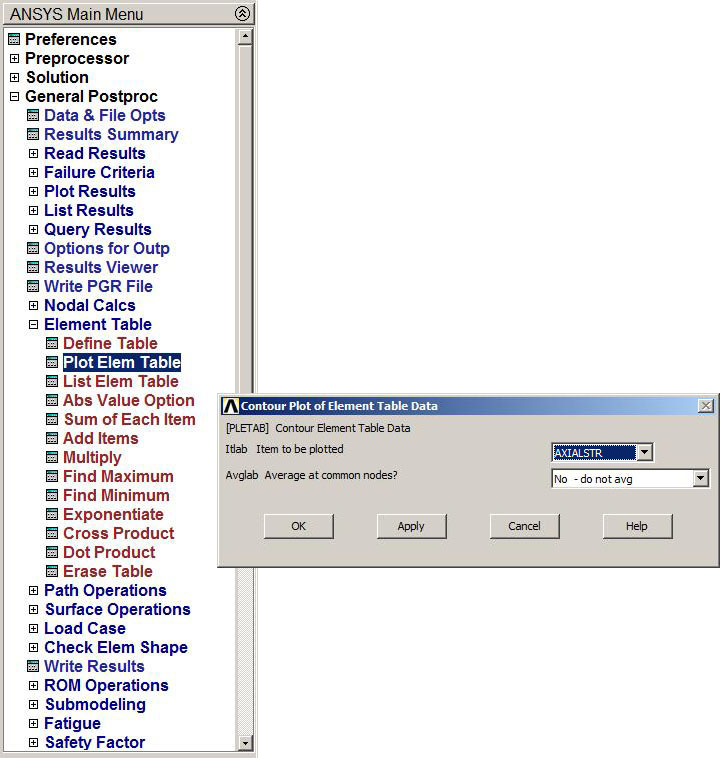
Figure 42. Element Table Data.
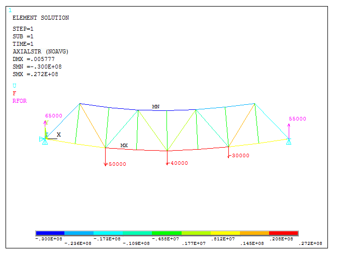
Figure 43. Plot deformations, stresses and external reactions.