PROBLEM
Figure 1 represents a three pinned bar structure of laminated steel. This structure supports a load of 70 kN.
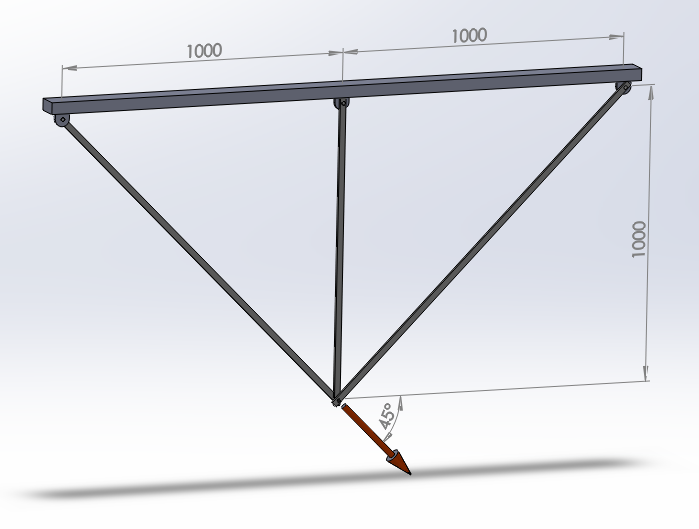
Figure 1. Three pinned bar structure.
Determine:
Tables 1 and 2 indicate the required data to solve this particular problem.
Table 1. Material properties.
| Steel | |
| Esteel | 210 GPa |
| Sy steel | 275 MPa |
| νsteel | 0.3 |
Table 2. Geometric characteristics for the bars.
| Geometric characteristics | |
| Section | 20 x 10 mm2 |
GEOMETRY OF THE MODEL
First of all, a name is defined for this problem, that is "Pinned bars" (Figure 2):
Utility Menu > File > Change Title
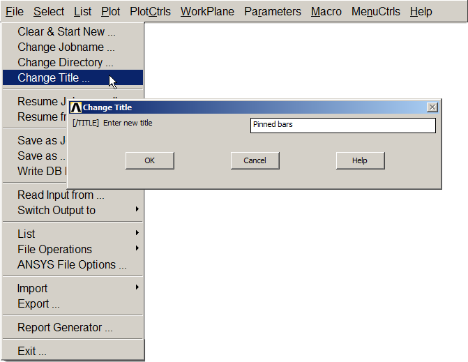
Figure 2. Change Title. "Pinned bars".
The title can be displayed with the option Replot:
Utility Menu > Plot > Replot
Now, it is defined the analysis as structural (Figure 3):
Main Menu > Preferences
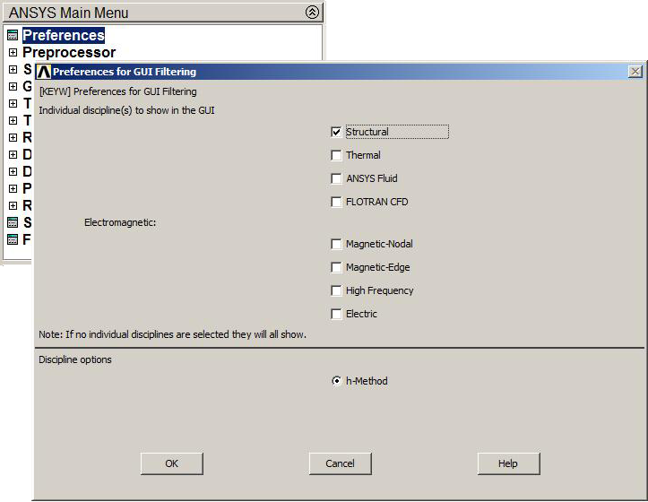
Figure 3. Structural analysis.
Then, LINK 180 element is selected for this particular problem, since the pinned bars are two-force members (Figure 4):
Main Menu > Preprocessor > Element Type > Add/Edit/Delete
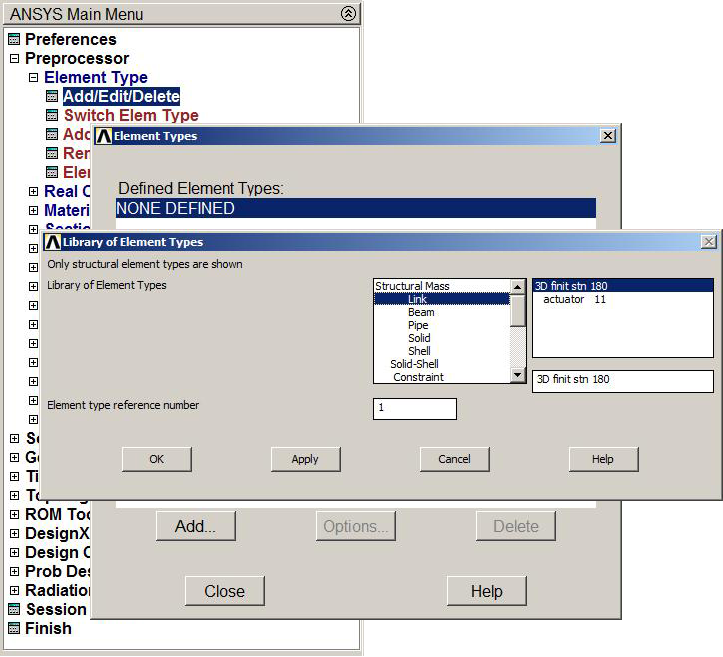
Figure 4. LINK 180 Element.
For this element type, real constants are required (Figure 5):
Main Menu > Preprocessor > Real Constants > Add
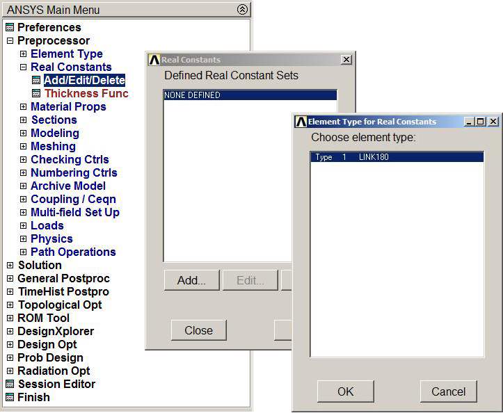 Figure 5. Real constants.
For LINK 180 element, the cross sectional area of the bar has to be defined (Figure 6):
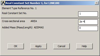
Figure 6. Cross sectional area.
It is worth saying that it is preferred to use the SI units. We need to define the material properties:
Main Menu > Preprocessor > Material Props > Material Models
For "Material Model Number 1" (Figure 7):
Material Model Number 1 > Structural > Linear > Elastic > Isotropic
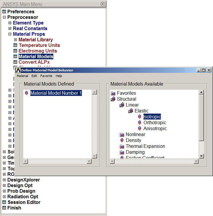
Figure 7. Material properties.
From the data provided by Table 1, we define the modulus of elasticity (EX) and the Poisson's ratio (PRXY) as indicated in Figure 8.
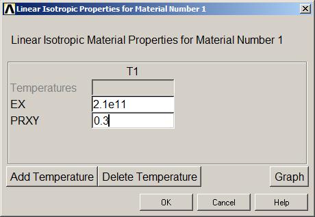
Figure 8. EX and PRXY definition.
To model the three bars, we start by defining four nodes (Figure 9):
Main Menu > Preprocessor > Modeling > Create > Nodes > In Active CS
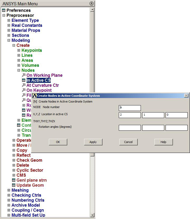
Figure 9. Create four nodes.
The coordinates for the four nodes are indicated in Table 3.
Table 3. Nodes
| NODE | X (m) | Y (m) |
| 1 | 1 | 0 |
| 2 | 0 | 1 |
| 3 | 1 | 1 |
| 4 | 2 | 1 |
Figure 10 is the graphic screen with the four nodes for the model.
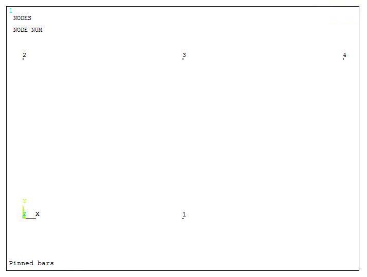
Figure 10. Graphic screen with the nodes.
Then, to create the bars (Figure 11):
Main Menu > Preprocessor > Modeling > Create> Elements > Auto Numbered > Thru Nodes
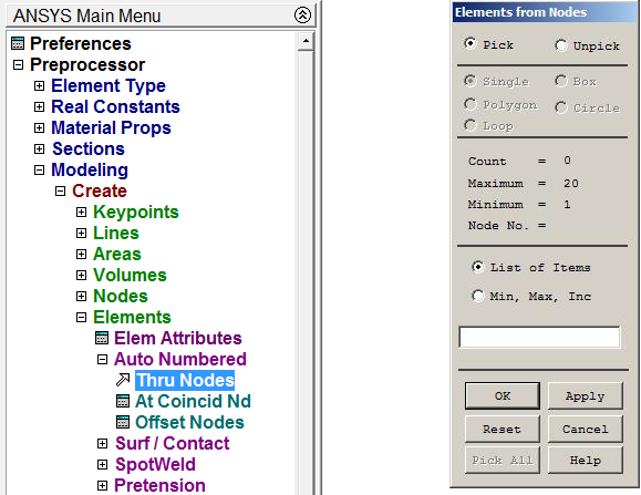
Figure 11. Create bars.
The process is to select nodes 1 and 2 and click on "Apply". Then, repeat the same process for the other bars and finally click on "OK".
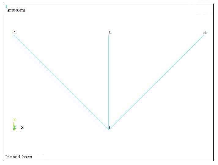
Figure 12. Graphic screen with the bars.
LOADS AND BOUNDARY CONDITIONS
The boundary conditions for this particular model are that the bars are restricted at nodes 2, 3 and 4. We select "All DOF" to restrict the displacements in UX, UY and UZ (Figure 13).
Main Menu > Preprocessor > Loads > Define Loads > Apply > Structural > Displacement > On Nodes
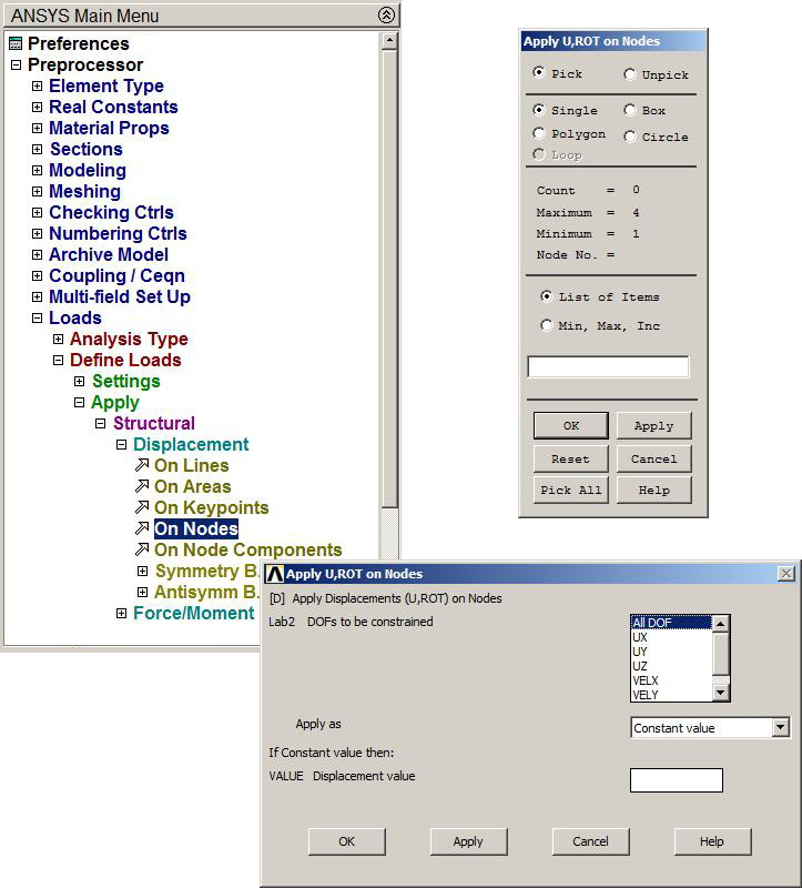
Figure 13. ALL DOF
The restrictions are represented in Figure 14.
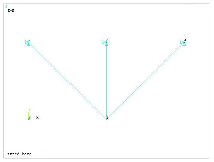
Figure 14. Graphic screen with restrictions.
To apply the load (Figure 15):
Main Menu > Preprocessor > Loads > Define Loads > Apply > Structural > Force/Moment > On Nodes
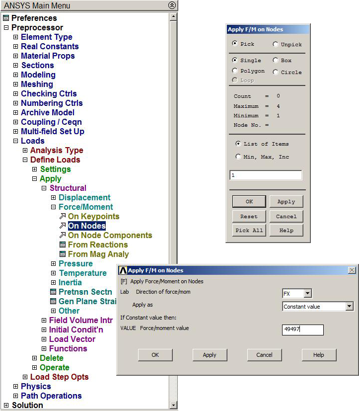
Figure 15. Applying the load.
Since the load has two components (FX and FY), it is necessary to calculate the two different values:
Fx = 70000 · cos(- 45) = 49497 N
Fy = 70000 · sin(- 45) = -49497 N
Figure 16 shows the graphic screen with the loads.
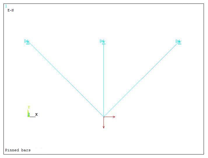
Figure 16. Applied force.
SOLUTION
Once the model has been created, we enter the "Solve" option:
Main Menu > Solution > Solve > Current LS
And Figure 17 shows the message "Solution is done!".
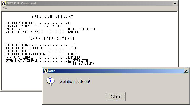
Figure 17. "Solution is done!".
RESULTS
In this stage of the problem, the first result to analyze is the deformation of the structure (Figure 18):
Main Menu > General Postprocessor > Plot Results > Deformed Shape
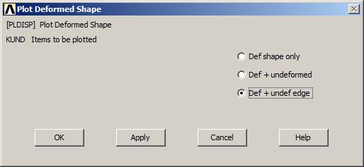
Figure 18. Option to analyze deformations.
Select the option "Def+undef edge". Figure 19 shows the graphic screen with the value for the maximum deformation (DMX), that is 0.0018 m.
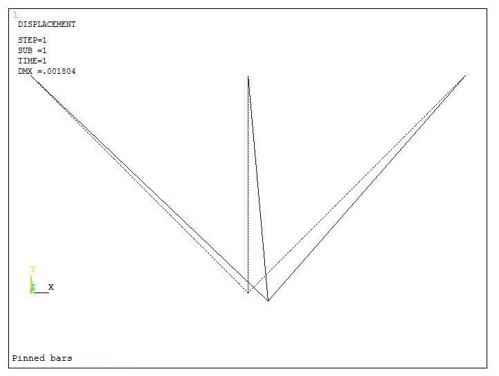
Figure 19. Deformation of the model.
Depending on the element type, some particular results can be obtained. Table 4 indicates some options for LINK 180 element. Each type of result has a particular label.
Table 4. Labels for LINK 180 element.
| AXIAL STRESS | LS, 1 |
| AXIAL DEFORMATION | LEPEL, 1 |
| AXIAL FORCE | SMISC, 1 |
For the results, it is necessary to define an Element Table Data (Figure 20):
Main Menu > General Postprocessor > Element Table > Define Table
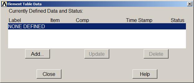
Figure 20. Defining an Element Table Data.
Click on "Add" to define additional element table items (Figure 21):
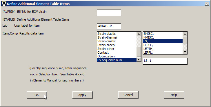
Figure 21. Additional Element Table Items.
In the "User Label" option, it is defined a name related with the result, in our case AXIALSTR. Next, click in "By Sequence Num" with the label. In this way, we define labels for deformations (AXIALDEF) and forces (AXIALFOR), as indicated in Figure 22.
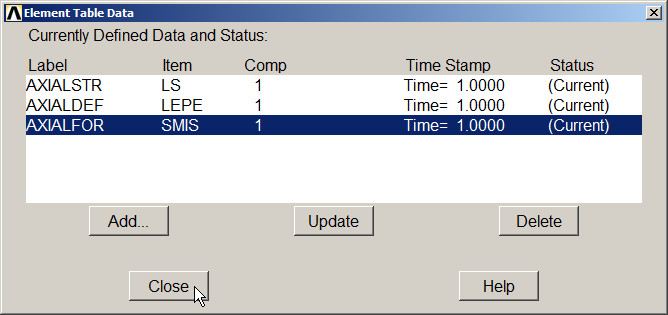
Figure 22. Element Table Data.
Then, to represent the stress distribution in each one of the bars, click on "Element Table > Plot Elem Table" (Figure 23):
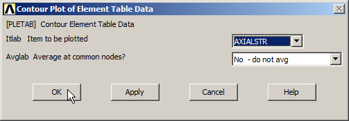
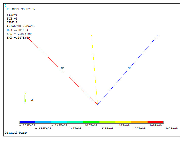
Figure 23. Stress distribution.
We can list the results from the option "List Element Table" (Figure 24):
Main Menu > General Postprocessor > Element Table > List Element Table
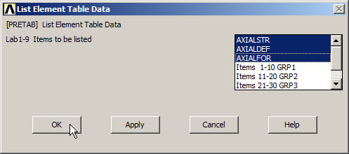
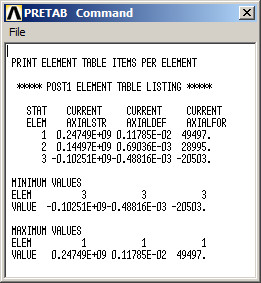
Figure 24. List Element Table.
Finally, to obtain the external reactions:
Main Menu > General Postprocessor > List Results > Reaction Solu
Select "All items" and the values for the external reactions appear in Figure 25.
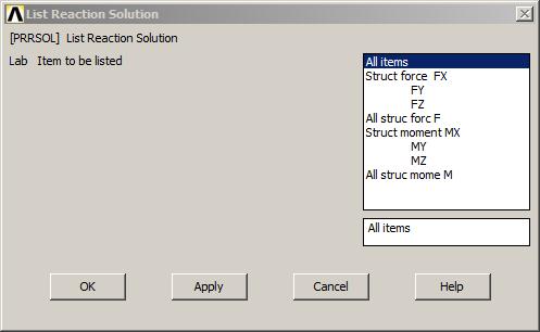
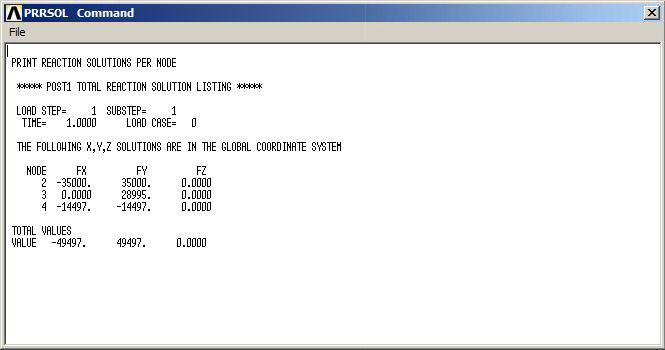
Figure 25. List Reaction Solution.
"Save Everything" from the Utility Menu.