
PROBLEM
Figure 1 shows a space frame truss.
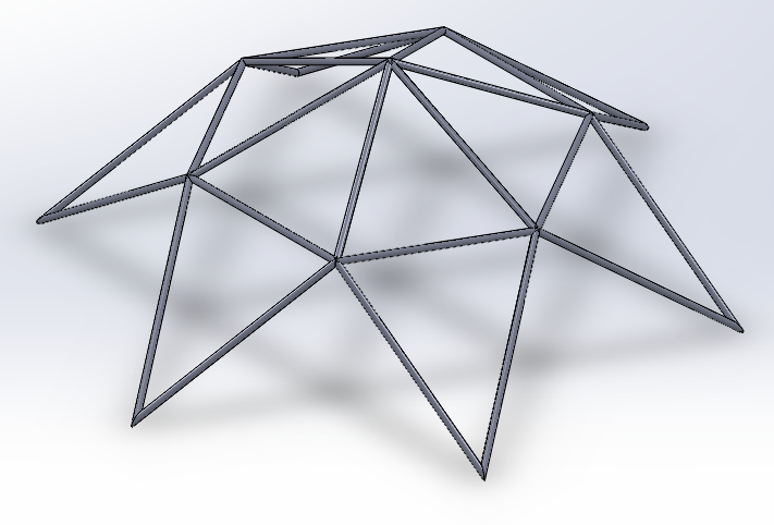
Figure 1a. Space frame truss.
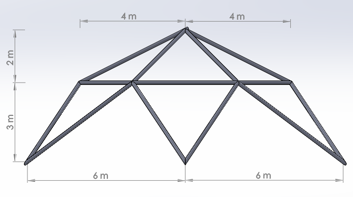
Figure 1b. Front view.

Figure 1c. Top view.
For each one of the load conditions determine:
Tables 1 and 2 indicate the properties of the material for the members and the two load conditions, respectively.
Table 1. Material Properties.
| Aluminium | |
| Ealuminium | 69 GPa |
| Sy aluminium | 210 MPa |
| νaluminium | 0.33 |
Table 2. Load Conditions.
| Applied loads | |||
| Load step 1 | Load step 2 | ||
| Node | FX(N) | Node | FY(N) |
| 1 | 2000 | 1 | 2000 |
| 2 | 1000 | 2 | 1000 |
| 3 | 1000 | 3 | 1000 |
| 4 | 1000 | 4 | 1000 |
| 5 | 1000 | 5 | 1000 |
| 6 | 1000 | 6 | 1000 |
| 7 | 1000 | 7 | 1000 |
GEOMETRY OF THE MODEL
First of all, we change the title for the problem (Figure 2):
Utility Menu > File > Change Title
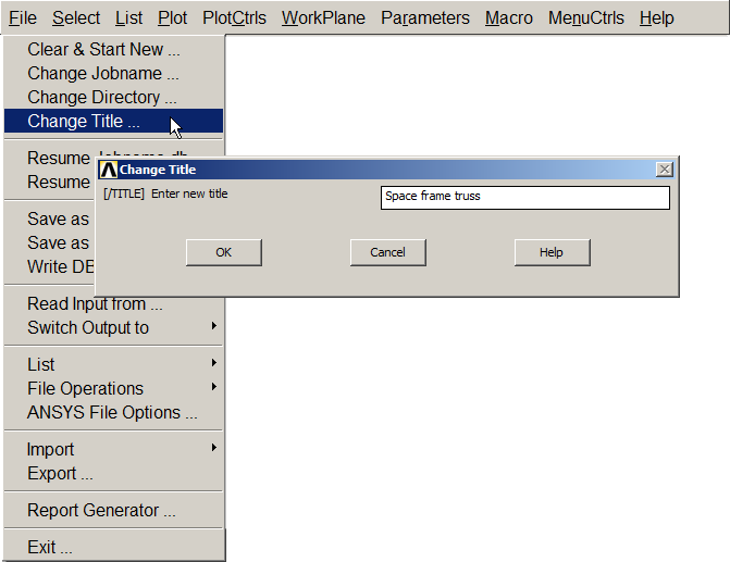
Figure 2. New title for the problem.
The Z-axis is defined in vertical position with the option "Z-axis up" (Figure 3):
Utility Menu > PlotCtrls > View Settings > Viewing Direction
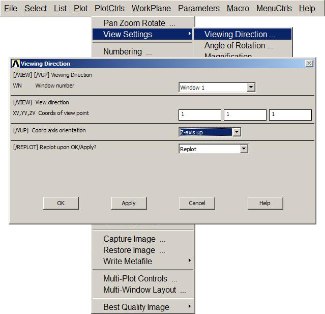
Figure 3. "Z-axis up".
Now, cylindrical coordinates are defined (Figure 4):
Utility Menu > WorkPlane > Change Active CS to > Global Cylindrical
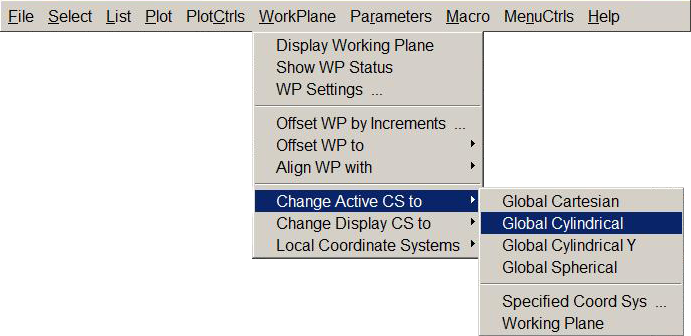
Figure 4. Global cylindrical coordinates.
And now angular units are defined. We select "Degrees DEG" (Figure 5):
Utility Menu > Parameters > Angular Units
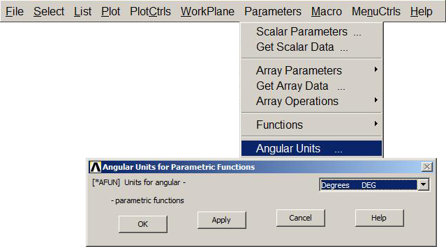
Figure 5. Angular units (degrees).
Since it is a structural problem, we can define this option (Figure 6):
Main Menu > Preferences > Structural
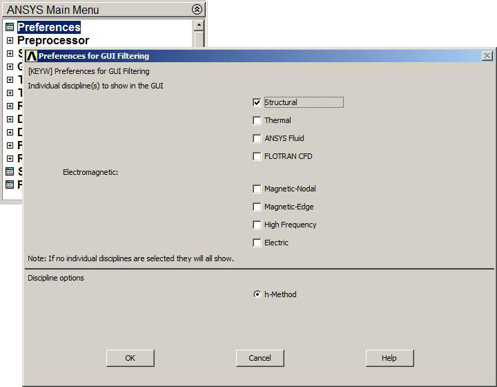
Figure 6. Structural analysis.
For this particular problem the element type "LINK 180" can be used, since it is an appropriate element for two-force members in three-dimension applications (Figure 7):
Main Menu > Preprocessor > Element Type > Add/Edit/Delete > LINK 180
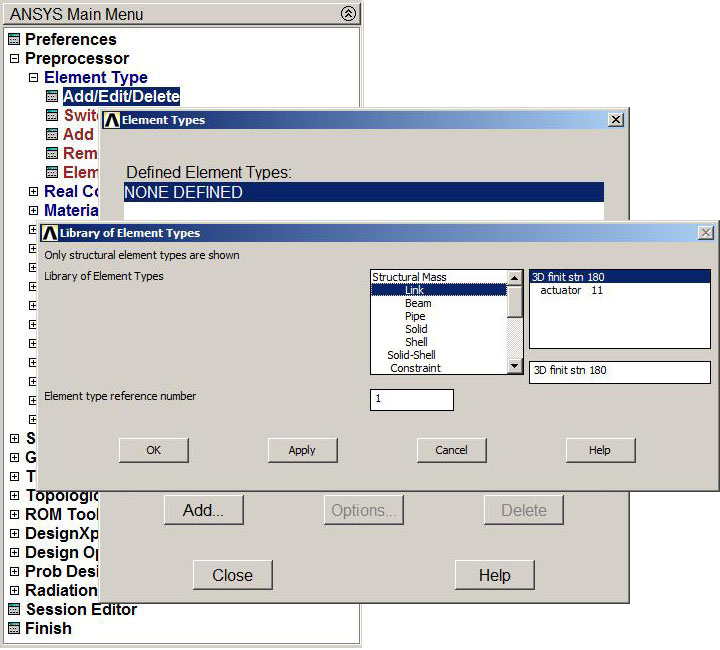
Figure 7. "LINK 180" element.
Next, we define the cross sectional area for the members (Figure 8):
Main Menu > Preprocessor > Real Constants > Add/Edit/Delete
Click on "LINK 180" and "OK". After that, define the area.
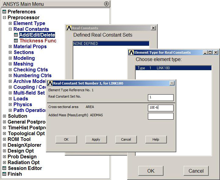
Figure 8. Cross sectional area.
Next, we have to define the properties of the material according to Table 1 (Figure 9):
Main Menu > Preprocessor > Material Props > Material Models
It is an isotropic material (Structural – Linear – Elastic – Isotropic).
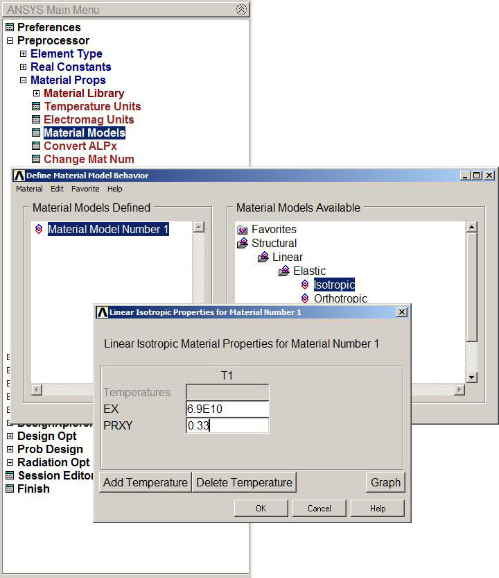
Figure 9. Modulus of elasticity (EX) and Poisson's ratio (PRXY).
Table 3 indicates the coordinates for the keypoints that define the space frame truss.
Table 3. Keypoints coordinates for the truss.
| Keypoint | X (m) | Y (degrees) | Z (m) |
| 1 | 0 | 0 | 5 |
| 2 | 4 | 90+60*0 | 3 |
| 3 | 4 | 90+60*1 | 3 |
| 4 | 4 | 90+60*2 | 3 |
| 5 | 4 | 90+60*3 | 3 |
| 6 | 4 | 90+60*4 | 3 |
| 7 | 4 | 90+60*5 | 3 |
| 8 | 6/cos(30) | 120+60*0 | 0 |
| 9 | 6/cos(30) | 120+60*1 | 0 |
| 10 | 6/cos(30) | 120+60*2 | 0 |
| 11 | 6/cos(30) | 120+60*3 | 0 |
| 12 | 6/cos(30) | 120+60*4 | 0 |
| 13 | 6/cos(30) | 120+60*5 | 0 |
Figure 10 shows the definition of the keypoint 13.
Main Menu > Preprocessor > Modeling > Create > Keypoints > In Active CS
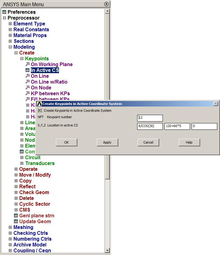
Figure 10. Keypoint 13.
Figure 11 represents the graphic screen with the keypoints.
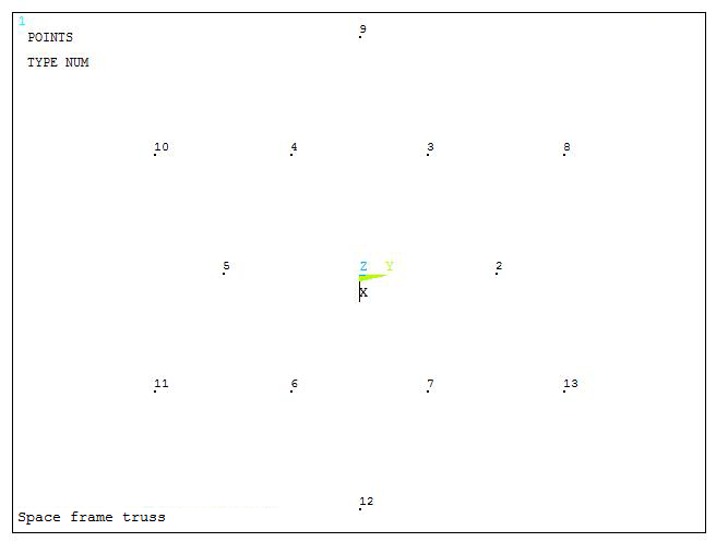
Figure 11. Graphic screen with the keypoints.
Lines between keypoints must be generated (Figure 12):
Main Menu > Preprocessor > Modeling > Create > Lines > Lines > Straight Line
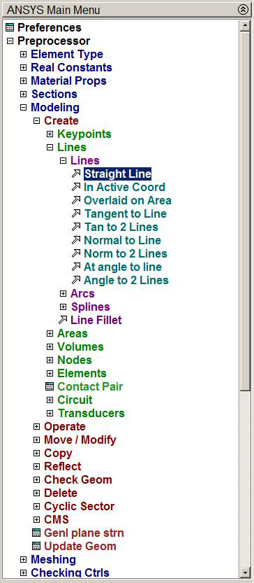
Figure 12. Creating lines between keypoints.
Figure 13 shows the top view of the truss.
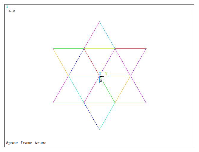
Figure 13. Top view of the truss.
And Figure 14 shows the truss in an isometric view.
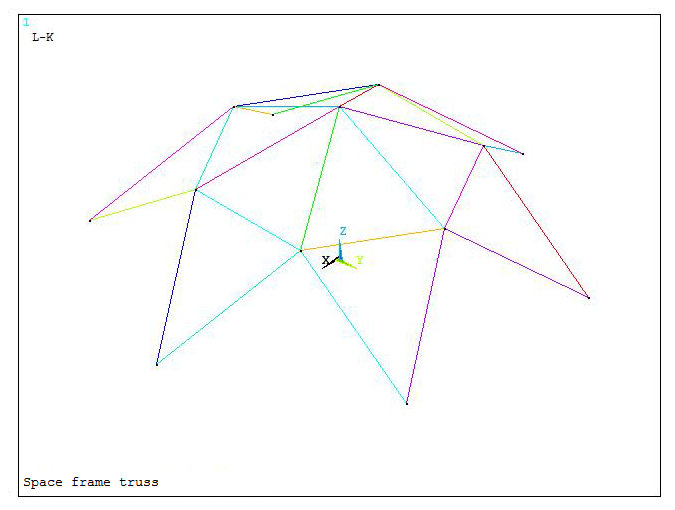
Figure 14. Isometric view of the truss.
Once the geometry of the space frame truss has been created, the next step is to mesh the members. Since they are two force members, the number of divisions for each member can be "1", because only axial forces act on the members (Figure 15):
Main Menu > Preprocessor > Meshing > Size Cntrls > ManualSize > Lines > All Lines
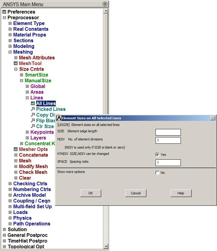
Figure 15. Element size to mesh the model.
To finish the meshing process (Figure 16):
Main Menu > Preprocessor > Meshing > Mesh > Lines > Pick All
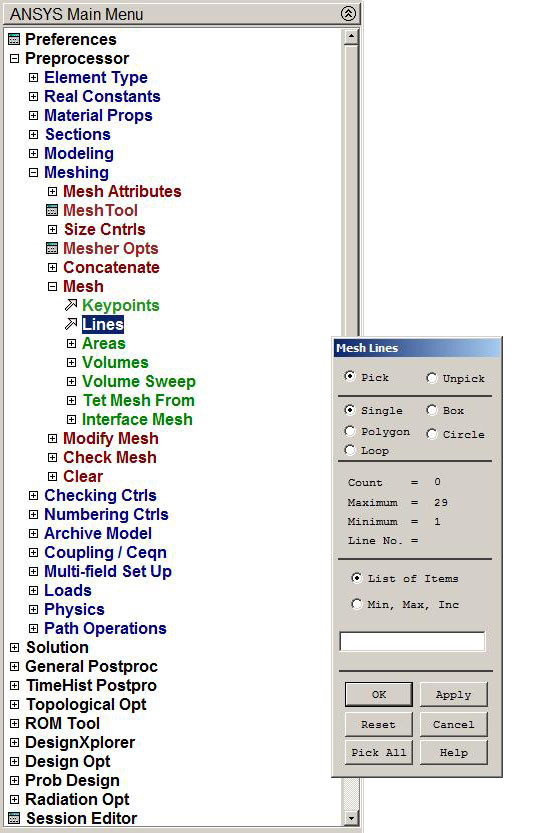
Figure 16. Meshing all lines.
Figure 17 represents the graphic screen with the model after the meshing process.
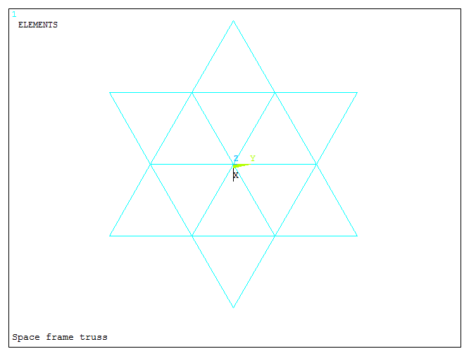
Figure 17. Meshed model.
LOADS AND BOUNDARY CONDITIONS
The next step is to define the boundary conditions for the model. The keypoints on the basis are fixed, so all degrees of freedom must be restricted ("All DOF" option in Figure 18):
Main Menu > Preprocessor > Loads > Define Loads > Apply > Structural > Displacement > On Keypoints > ALL DOF
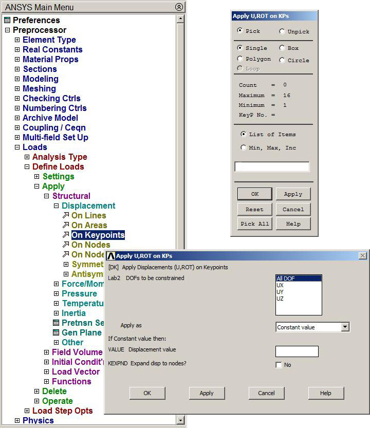
Figure 18. "All DOF" option for keypoints.
Now, forces are applied. According to the first load condition (Table 2) the forces are acting in the X-direction (Figure 19).
Main Menu > Preprocessor > Loads > Define Loads > Apply > Structural > Force/Moment > On Keypoints
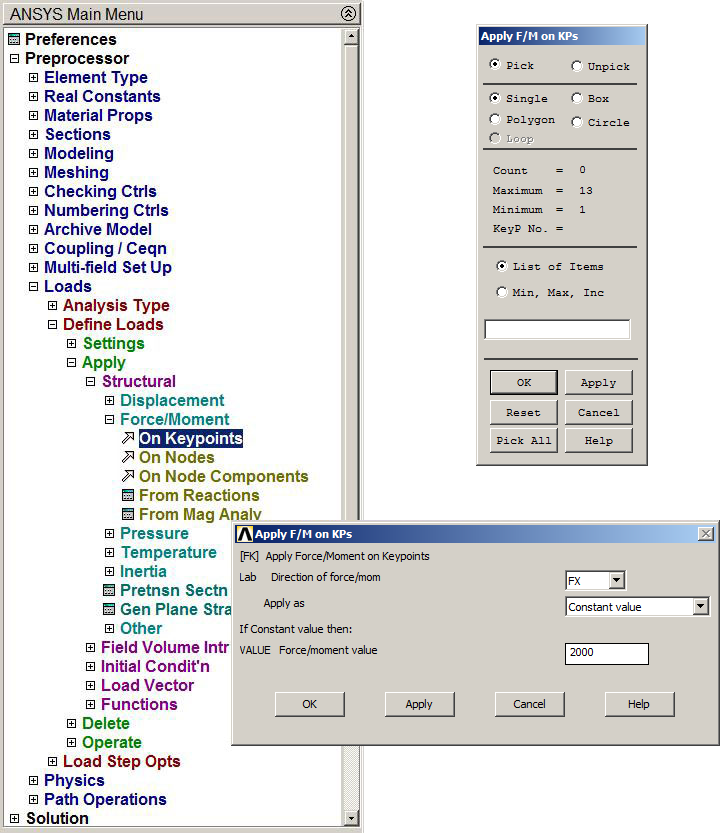
Figure 19. Defining forces in X-direction.
Figure 20 represents the graphic screen with the applied forces in X-direction.
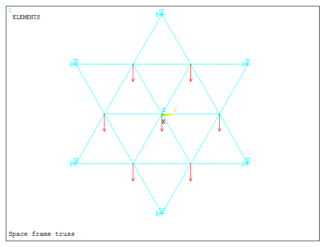
Figure 20. Graphic screen with forces in X-direction.
The first load condition must be saved as "1" (Figure 21):
Main Menu > Solution > Load Step Opts > Write LS File
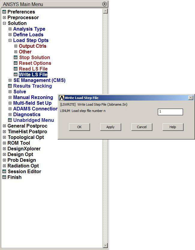
Figure 21. "Write Load Step File" for first load condition.
Now, we define the second load condition after deleting the first one (Figure 22):
Main Menu > Preprocessor > Loads > Define Loads > Delete > Structural > Force/Moment > On Keypoints
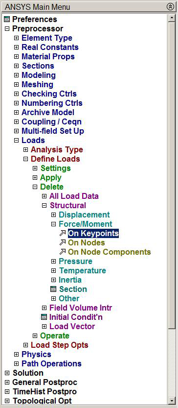
Figure 22. Delete first load condition.
For the second load condition, forces in Y-direction must be defined (Figure 23):
Main Menu > Preprocessor > Loads > Define Loads > Apply > Structural > Force/Moment > On Keypoints

Figure 23. Defining forces in Y-direction.
Figure 24 represents the graphic screen with forces acting in Y-direction.
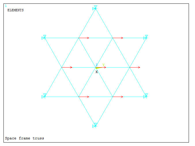
Figure 24. Graphic screen with forces in Y-direction.
The second load condition must be saved as "2" (Figure 25).
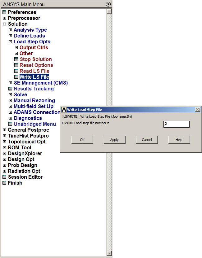
Figure 25. "Write Load Step File" for second load condition.
SOLUTION
After the loads and boundary conditions have been defined, the space frame truss is solved (Figure 26):
Main Menu > Solution > Solve > From LS Files
In the window "Solve Load Step Files", we define the solution process from first load condition "1" (LSMIN) to second load condition "2" (LSMAX) with an increment of "1" (LSINC).
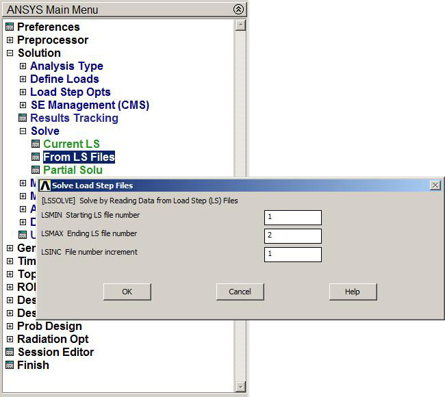
Figure 26. Solve Load Step Files.
RESULTS
After the solution process, results can be analyzed. First of all, we look at the deformation (Figure 27):
Main Menu > General Postproc > Plot Results > Deformed Shape
The option "Def+undef edge" is selected.
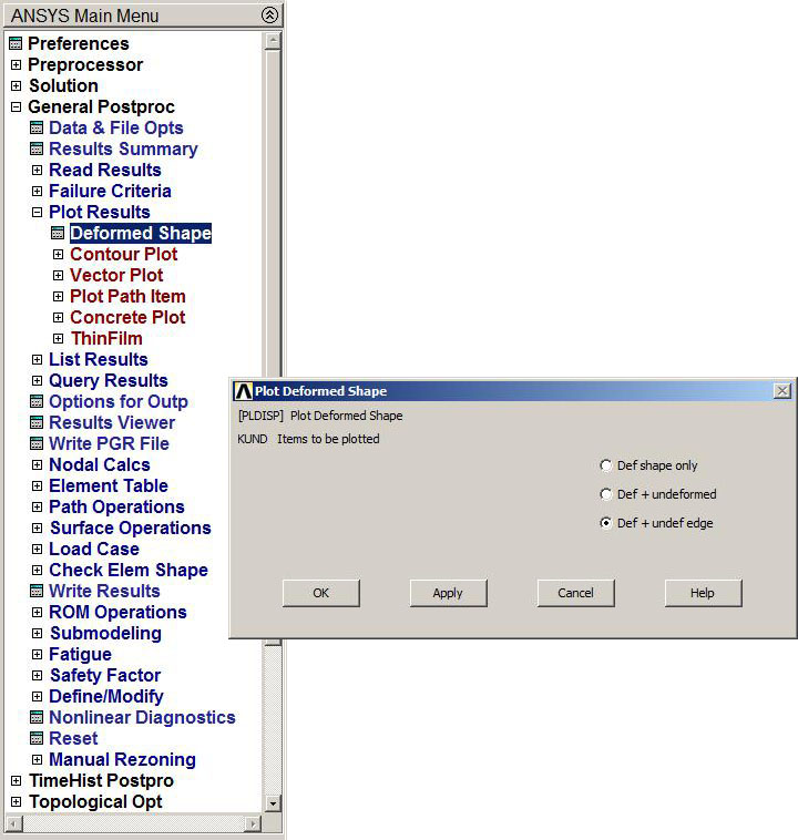
Figure 27. "Def+undef edge" option.
Figure 28 represents the graphic screen with the deformation for the truss.
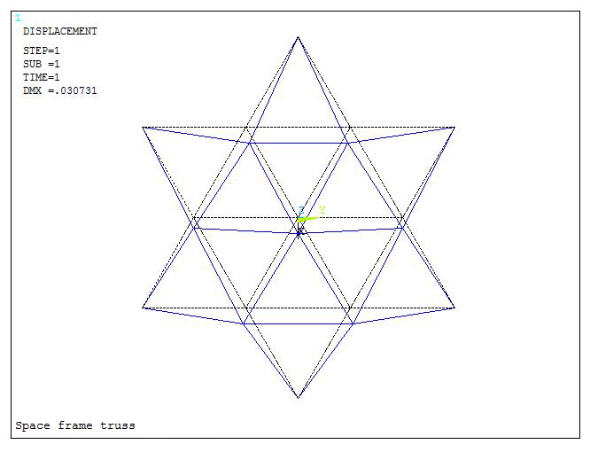
Figure 28. Deformation for the truss.
The other result to evaluate is the stress distribution in members. First of all, each member is going to be numbered with the "Numbering" option (Figure 29):
Utility Menu > PlotCtrls > Numbering
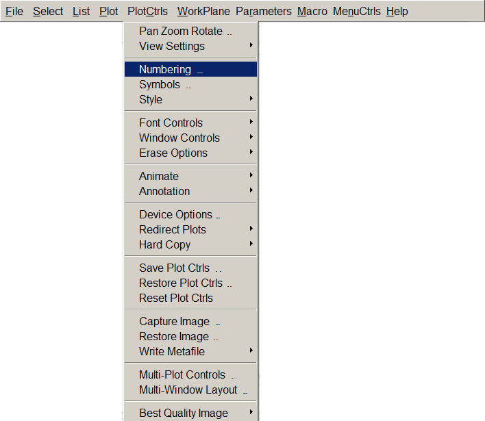
Figure 29. Numbering members.
We select "Element numbers" (Figure 30):
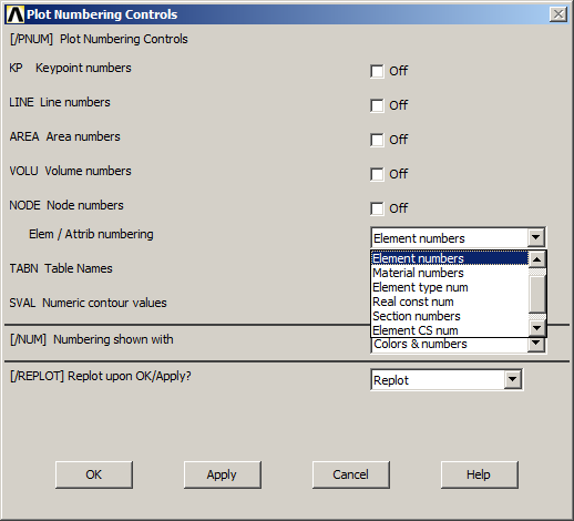
Figure 30. "Element numbers" option.
Figure 31 represents the graphic screen with every member numbered.
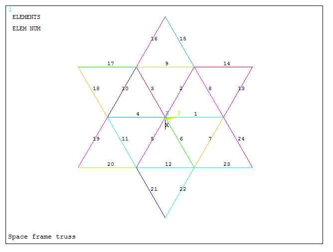
Figure 31. Numbered members.
To evaluate the stresses, a table must be defined:
Main Menu > General Postproc > Element Table > Define Table
In the window "Define Additional Element Table Items", we define a new label for axial stresses (AXIALSTR) and then we activate "By sequence num" and "LS, 1", as indicated in Figure 32:
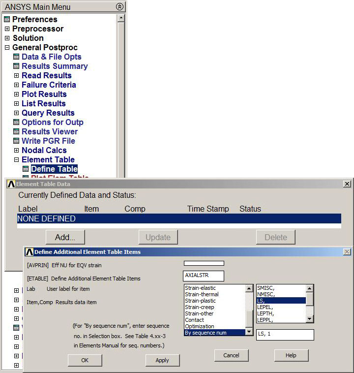
Figure 32. Define Element Table.
For axial forces, the label is "AXIALFOR" and for "By sequence num" we select "SMISC, 1" (Figure 33).
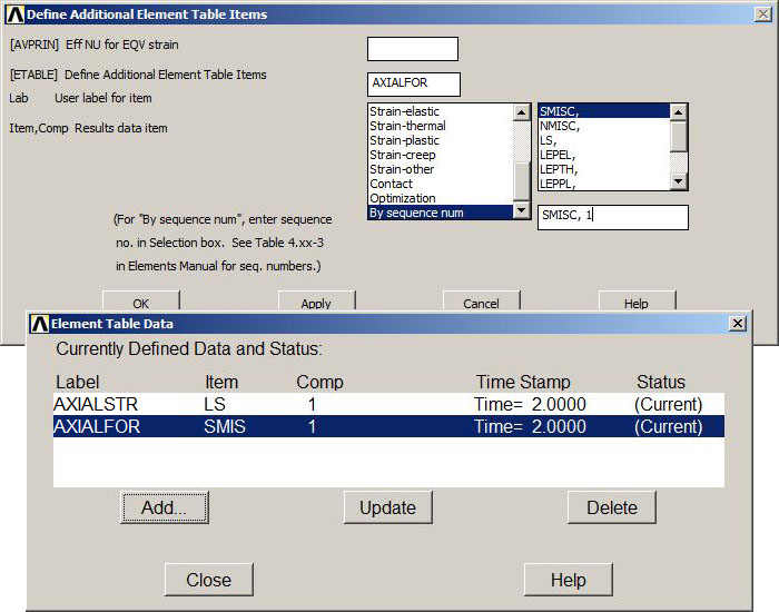
Figure 33. Element Table Data.
To obtain the results, the two labels must be selected from "Elem Table Data" (Figure 34):
Main Menu > General Postproc > List Results > Elem Table Data
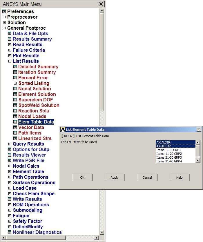
Figure 34. Select labels form Element Table Data.
Results are listed in Figure 35.
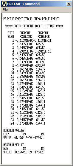
Figure 35. List of results.
Finally, the results can be plotted as indicated in Figure 36:
Main Menu > General Postproc > Element Table > Plot Elem Table
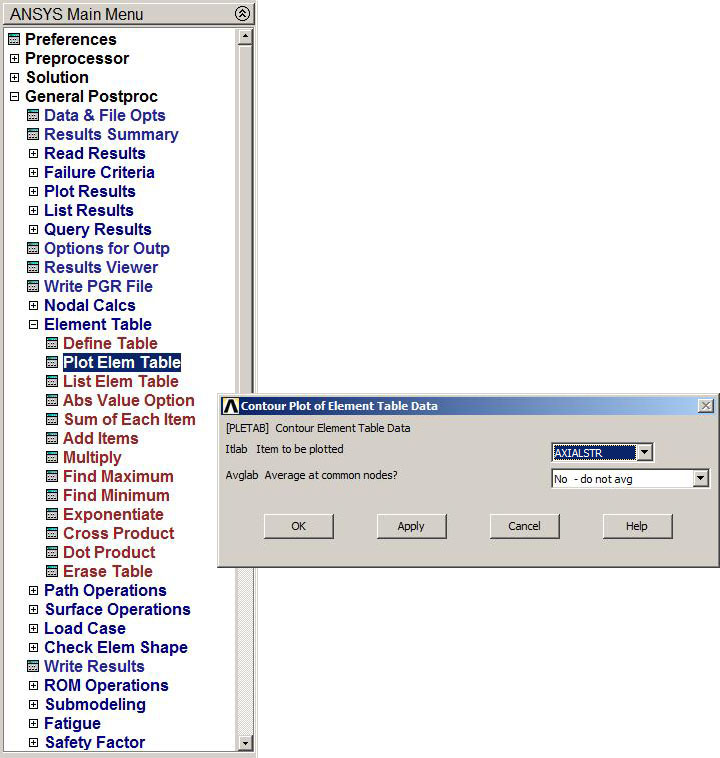
Figure 36. Select "AXIALSTR".
Figure 37 represents the graphic screen with the stress distribution in the truss.

Figure 37. Stress distribution.
To evaluate the results for the second load condition (Figure 38):
Main Menu > General Prostproc > Read Results > Next Set
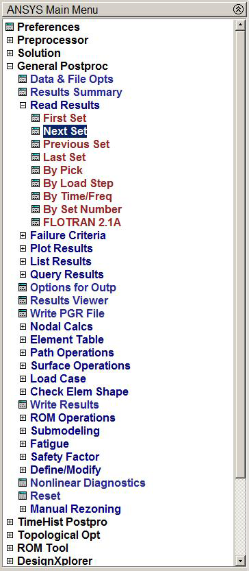
Figure 38. "Next set" for the second load condition.
Figure 39 represents the deformation of the truss for the second load condition.
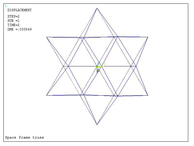
Figure 39. Deformation of the truss. Second load condition.
Now we can obtain the stress distribution for the second load condition (Figure 40) selecting "UPDATE" from:
Main Menu > General Prostproc > Element Table > Define Table
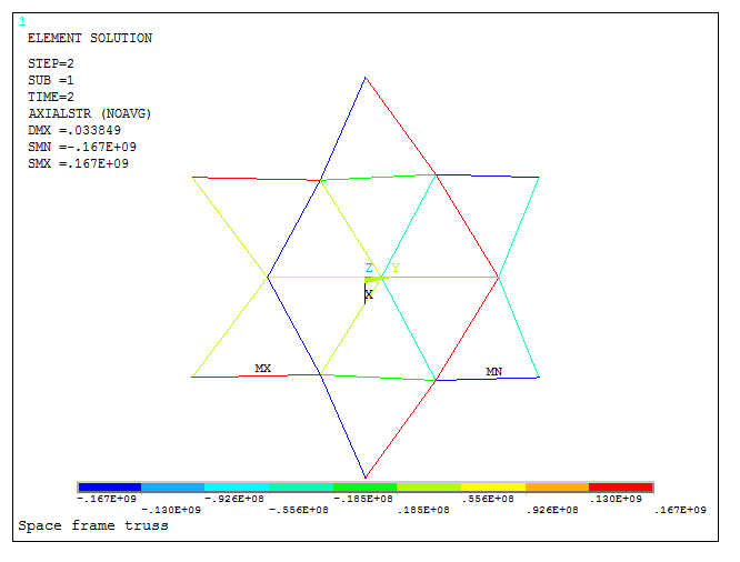
Figure 40. Stress distribution. Second load condition.
Finally, the results are listed in the same way as for the first load condition (Figure 41).
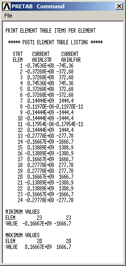
Figure 41. Results for the second load condition.
It is observed that the maximum force is 1764.1 N (first load condition). So, the minimum cross sectional area is: A = 1764.1 / 210·106 = 8.4·10-6 m2 = 8.4 mm2.