PROBLEM
Figure 1 shows a Fink Truss. Calculate the maximum deformation, the external reactions and the maximum value of stress.

Figure 1. Fink truss.
Table 1 indicates the mechanical properties of the laminated steel for the members of the truss, and Table 2 indicates the geometric characteristics of the two types of bars used for this particular problem.
Table 1. Material properties.
| Steel S 275 JR | |
| Esteel | 210 GPa |
| Sy steel | 275 MPa |
| νsteel | 0.3 |
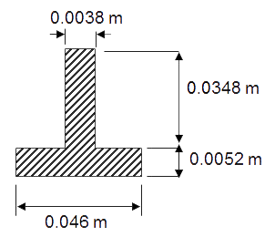
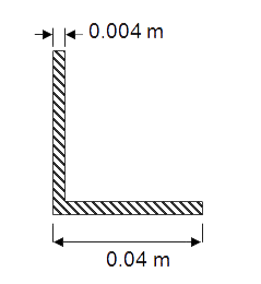
Table 2. Geometric characteristics.
| Cross sections | |
| T40 | L40x4 |
 |
 |
GEOMETRY OF THE MODEL
First of all, define a name for the problem. In this example, "Fink truss". (Figure 2).
Utility Menu > File > Change Title
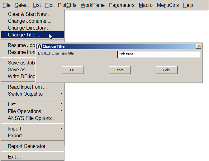
Figure 2. Change Title.
Define the problem as "Structural" (Figure 3).
Main Menu > Preferences > Structural
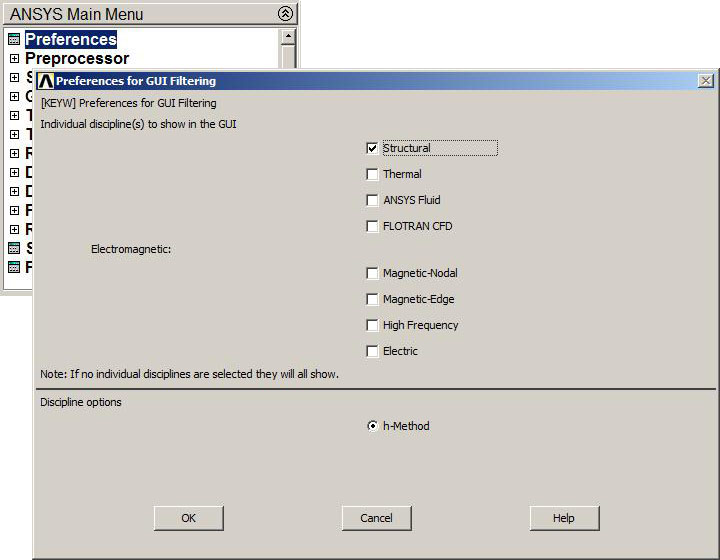
Figure 3. "Structural analysis".
The element type is "BEAM 2 node 188" (Figure 4).
Main Menu > Preprocessor > Element Type > Add/Edit/Delete
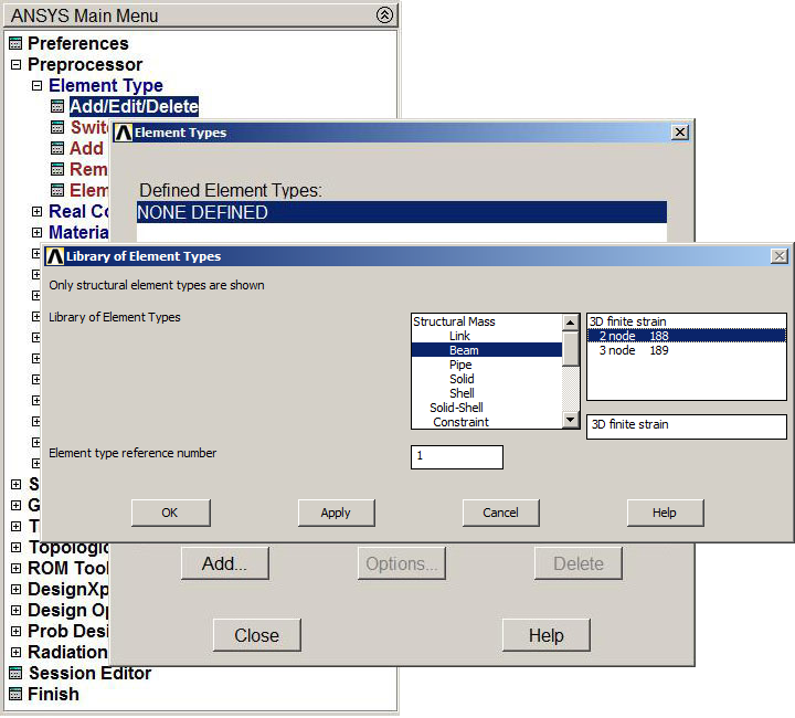
Figure 4. Element "BEAM 2 node 188".
Define the mechanical properties of the steel (Figure 5):
Main Menu > Preprocessor > Material Props > Material Models
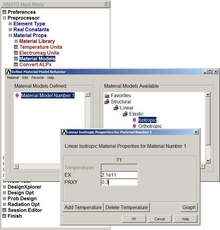
Figure 5. Material properties.
Define the cross sections. First the T40 section, as indicated in Table 2. (Figure 6).
Main Menu > Preprocessor > Sections > Beam > Common Sections
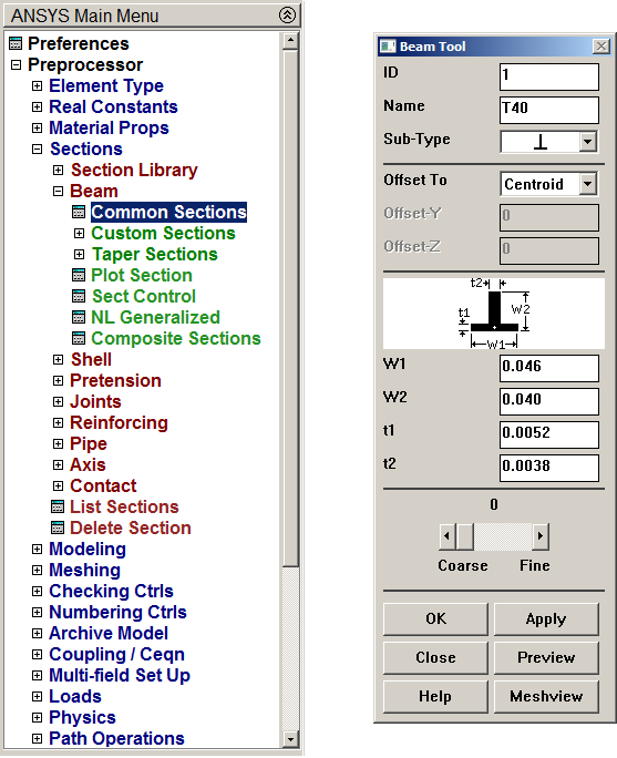
Figure 6. T40 section.
Plot the geometric characteristics of this section (Figures 7 and 8).
Main Menu > Preprocessor > Sections > Beam > Plot Section
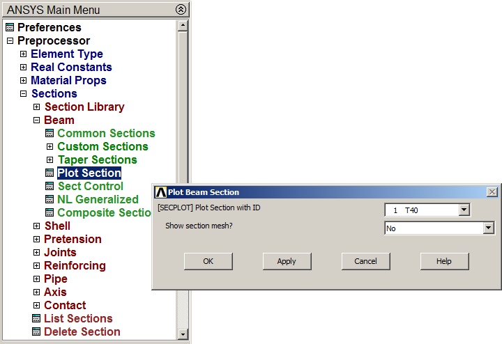
Figure 7. Plot Section.
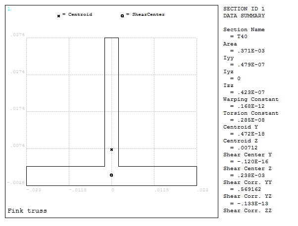
Figure 8. Geometric characteristics of the T40 section.
Now, read the L40x4 section (see "Custom Sections") as indicated in Figure 9.
Main Menu > Sections > Beam > Custom Sections > Read Sect Mesh
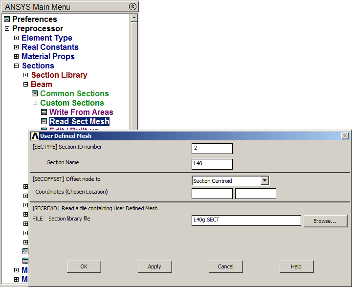
Figure 9. Read "L40g.SECT" file.
Plot the L40x4 section (Figure 10).
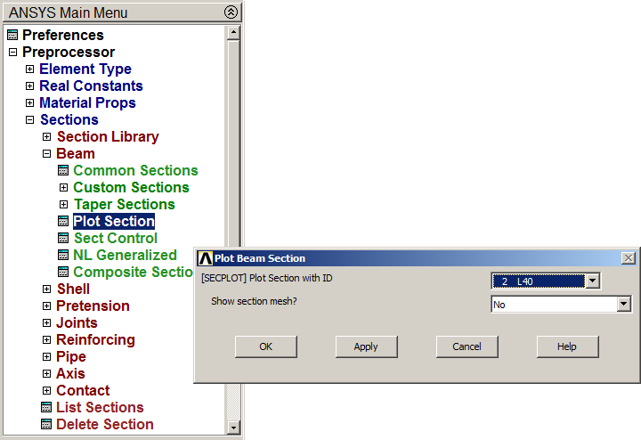
Figure 10. "Plot Beam Section".
Figure 11 shows the geometric characteristics of the L40x4 section.
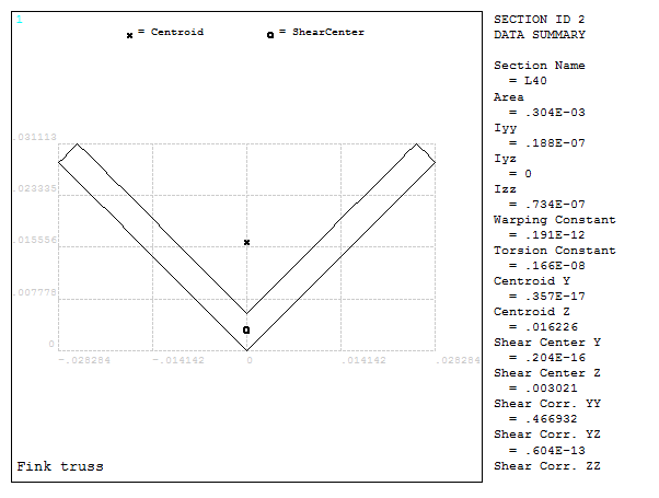
Figure 11. Geometric characteristics of the L40x4 section.
Create the keypoints from the coordinates that are indicated in Table 3.
Main Menu > Preprocessor > Modeling > Create > Keypoints > In Active CS
Table 3. Keypoints coordinates.
| Keypoint | X (m) | Y (m) | Z (m) |
| 1 | 0 | 0 | 0 |
| 2 | 1 | 0 | 0 |
| 3 | 2 | 0 | 0 |
| 4 | 2.5 | 0 | 0 |
| 5 | 3 | 0 | 0 |
| 9 | 0 | 1.5 | 0 |
Create the six keypoints as indicated in Figure 12.
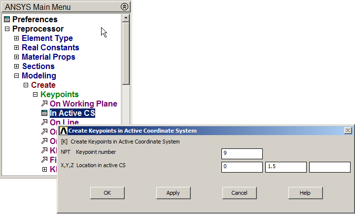
Figure 12. Creating keypoint 9.
Figure 13 represents the keypoints.
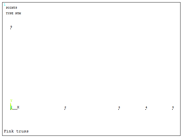
Figure 13. Keypoints.
Create lines between the keypoints (Figure 14).
Main Menu > Preprocessor > Modeling > Create > Lines > Lines > Straight Line
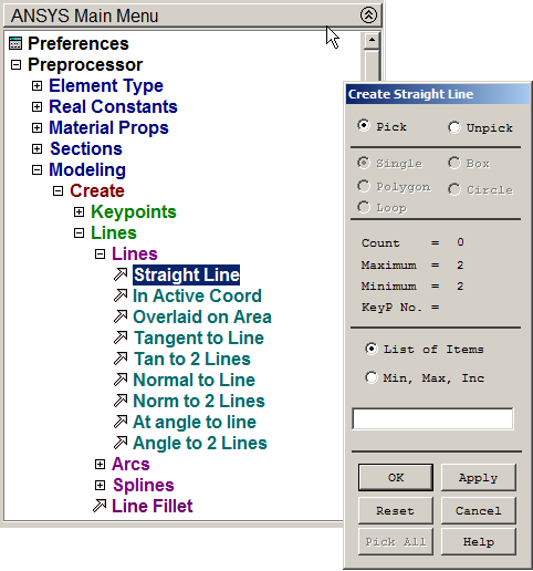
Figure 14. Creating lines.
Lines are defined according to Table 4.
Table 4. Lines.
| Line | First keypoint | Second keypoint |
| 1 | 1 | 2 |
| 2 | 2 | 3 |
| 3 | 3 | 4 |
| 4 | 4 | 5 |
| 5 | 5 | 9 |
The inclined member is divided in four lines (Figure 15):
Main Menu > Preprocessor > Modeling > Operate > Booleans > Divide > Line into N Ln's
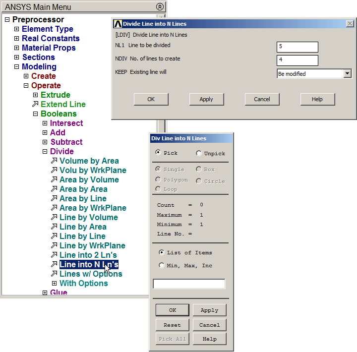
Figure 15. Divide line 5.
Figure 16 represents the graphic screen with the divisions for the inclined member. First, number the keypoints:
Utility Menu > PlotCtrls > Numbering
Click "On" for "Keypoints numbers".
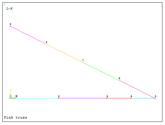
Figure 16. Diagonal member division.
Define a new line between keypoints 2 and 9 and divide it in two lines to obtain the keypoint 10 (Figure 17). Then, create the other lines.

Figure 17. Divide the line between keypoints 2 and 9.
Figure 18 shows the lines and keypoints that have been created.
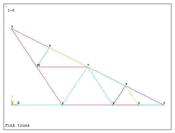
Figure 18. Lines and keypoints.
Now, copy the structure with the option "Reflect", as indicated in Figure 19.
Main Menu > Preprocessor > Modeling > Reflect > Lines
Click "Pick All".
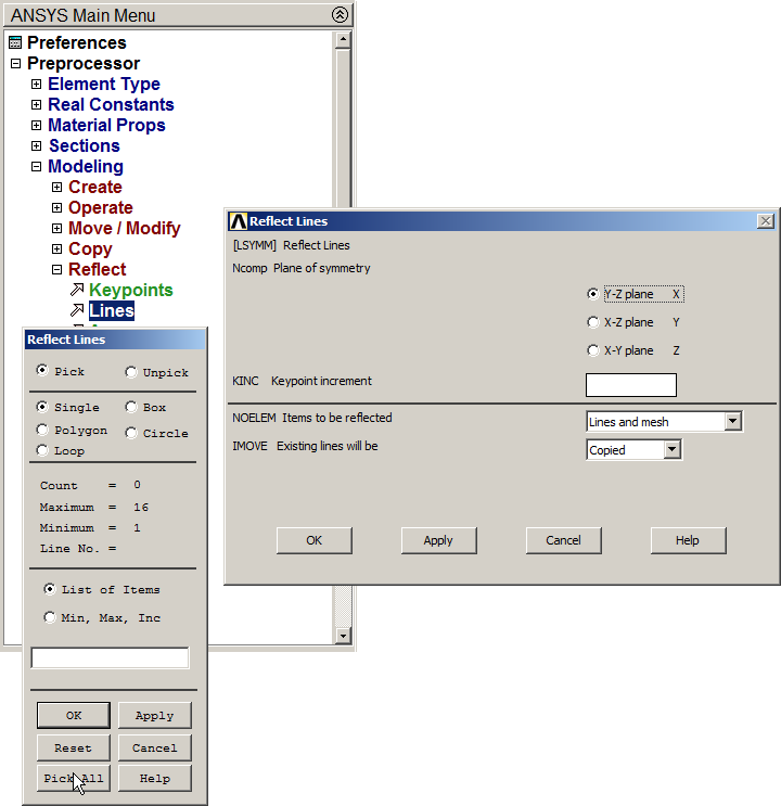
Figure 19. Option "Reflect Lines".
Figure 20 represents the complete structure, that is a Fink truss.

Figure 20. Defined Fink truss.
Now, to avoid the duplicity of keypoints, use the option "Merge items", as indicated in Figure 21.
Main Menu > Preprocessor > Numbering Ctrls > Merge Items
And select "keypoints" in "Type of item to be merge".
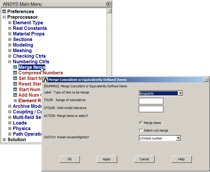
Figure 21. Merge Keypoints.
After that, mesh the lines. First, assign section T40 (Figure 22).
Main Menu > Preprocessor > Meshing > Mesh Attributes > Picked Lines
Select the corresponding lines for this section.
To define the right orientation for sections, activate "Pick Orientation Keypoint(s)". For this particular problem, T40 sections have to be oriented toward the interior of the truss.

Figure 22. Line Attributes for T40 section.
Now select a keypoint previously defined or, alternatively, create it, which is contained in the plane (in this case, the XY plane), in which the section is oriented (look at "BEAM Element 188" in ANSYS Help). Keypoint 10 is the required point.
Then, assign L40 section in the same way as before for the corresponding lines (Figure 23).
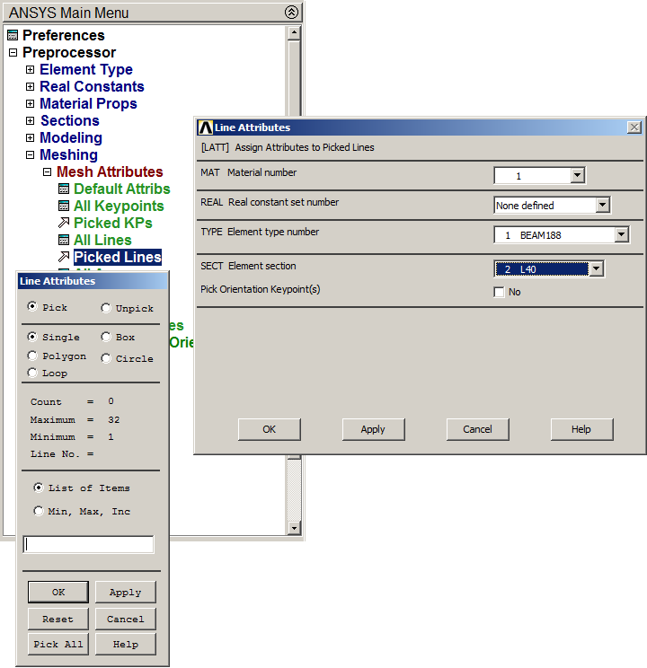
Figure 23. Line Attributes for L40 section.
Next, mesh the lines. The element size is 0.1 m (Figure 24).
Main Menu > Preprocessor > Meshing > Size Cntrls > Manual Size > Lines > All Lines

Figure 24. Element size of 0.1 m.
Finish the meshing process (Figure 25).
Main Menu > Preprocessor > Meshing > Mesh > Lines
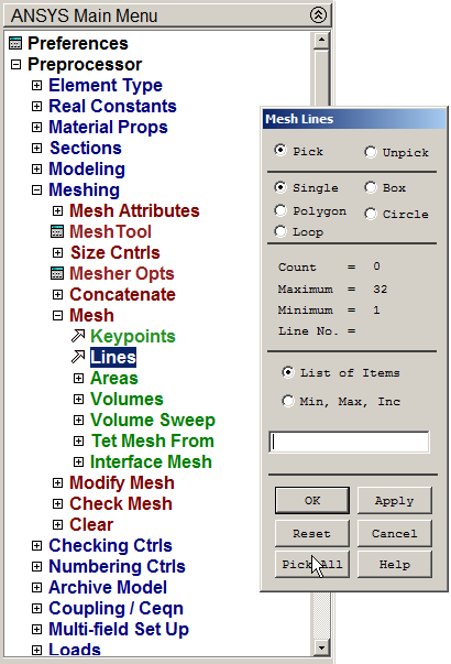
Figure 25. Mesh Lines.
The option "Display of element" is used to represent the 3D model. (Figure 26):
Utility Menu > PlotCtrls > Style > Size and Shape
Activate "On" in ESHAPE.
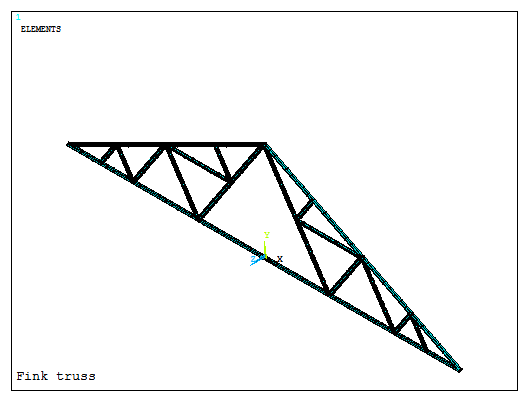
Figure 26. 3D model of the truss.
The option "Pan-Zoom-Rotate" from PlotCtrls menu can be used to approach a particular part of the model. Click "Box zoom" and select one part of the model as indicated in Figure 27.
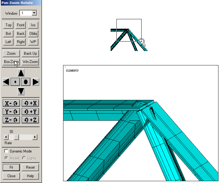
Figure 27. The option "Pan-Zoom-Rotate".
LOADS AND BOUNDARY CONDITIONS
According to Figure 1, the left end of the structure is pinned, and the right end is simply supported. It is worth saying that displacement in Z direction must be restricted to avoid torsion, since this is a 3D model. Figure 28 indicates the restriction for the left end.
Main Menu > Preprocessor > Loads > Define Loads > Apply > Structural > Displacement > On Keypoints
Select "UX", "UY", "UZ" and "ROTX".
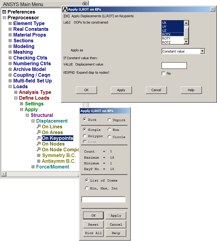
Figure 28. Boundary condition for the left support.
In the same way, define the conditions for the right end as indicated in Figure 29.
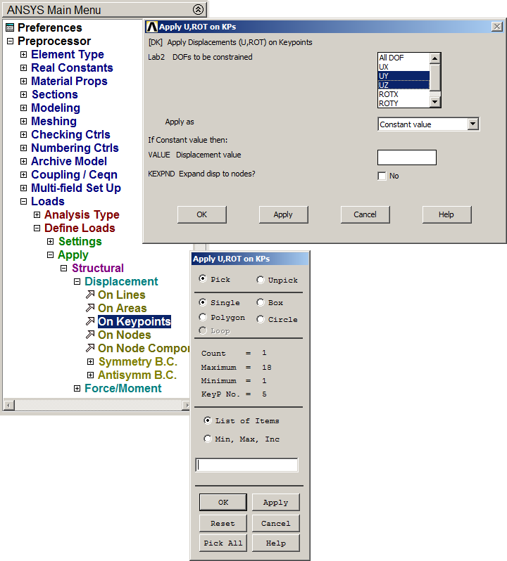
Figure 29. Boundary condition for the right support.
Next, apply the loads acting on the truss. Figure 30 shows the application of the 20000 N loads.
Main Menu > Preprocessor > Loads > Define Loads > Apply > Structural > Force/Moment > On Keypoints
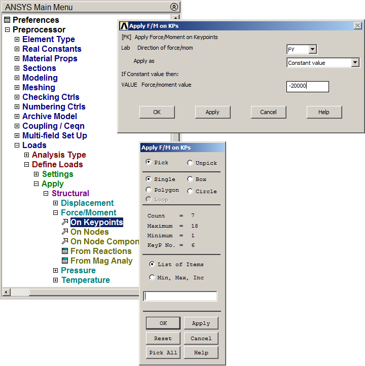
Figure 30. Applying 20000 N loads.
And Figure 31 indicates the application of the 10000 N loads.
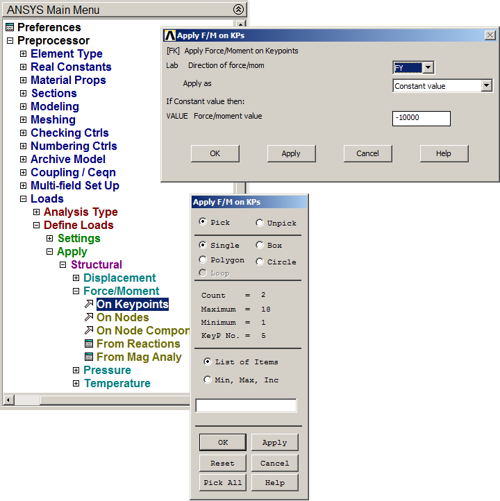
Figure 31. Applying 10000 N loads.
SOLUTION
Once the model has been defined, solve the problem:
Main Menu > Solution > Solve > Current LS
After "Solution is done!" message, click "OK".
RESULTS
First, analyze the deformation of the truss (Figure 32).
Main Menu > General Postproc > Plot Results > Contour Plot > Nodal Solu
And select the option "Displacement vector sum".
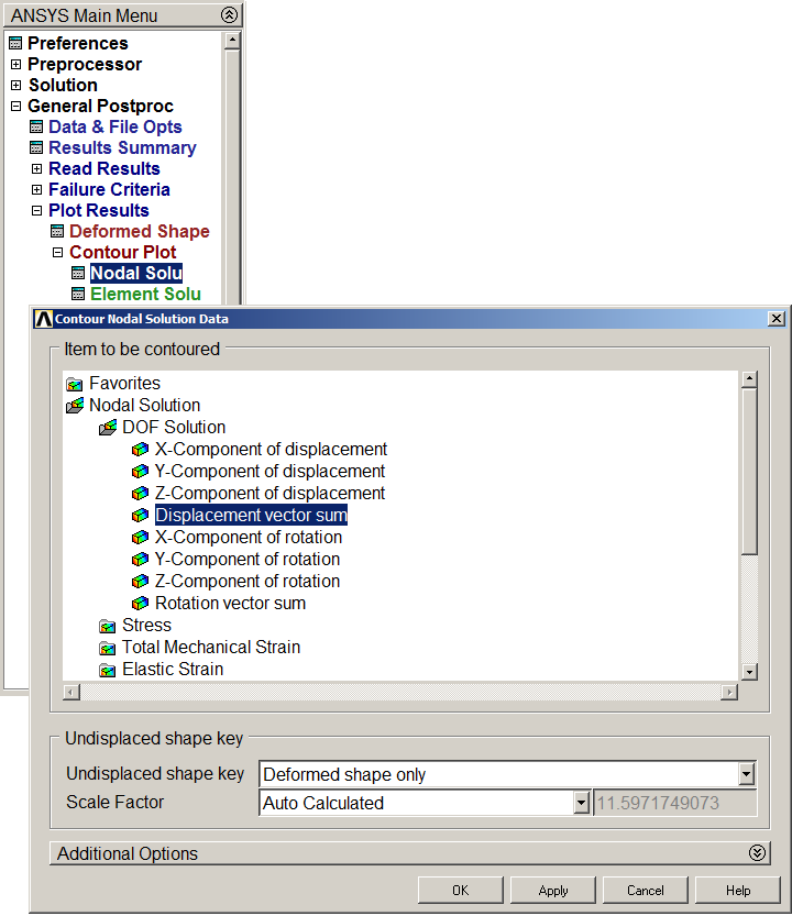
Figure 32. "Displacement vector sum".
Figure 33 represents the deformation of the model.
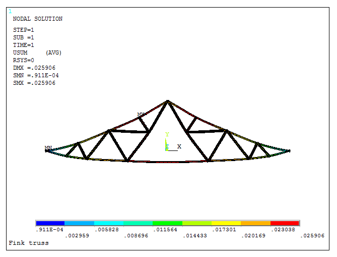
Figure 33. Deformation of the model.
Activate the options indicated in Figure 34 to represent the values of the forces and reactions.
Utility Menu > PlotCtrls > Symbols
Select "For Individual" and "OK".
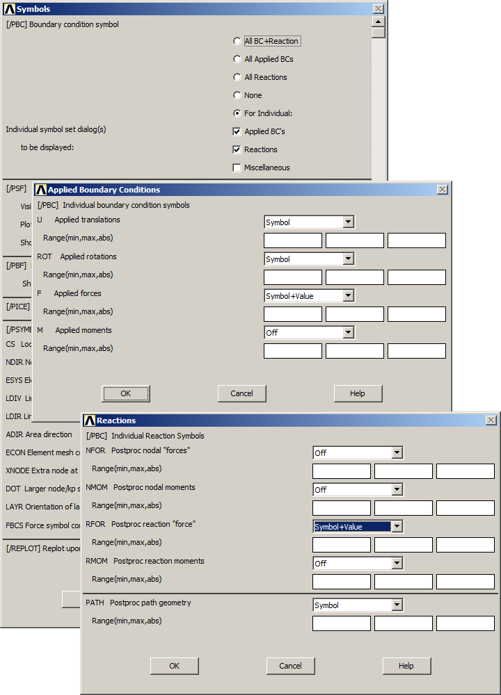
Figure 34. Activate symbols for results.
Now, Figure 35 shows the deformation of the truss and the external reactions.
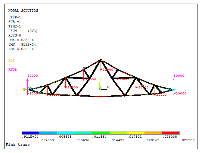
Figure 35. Deformation and external reactions.
Finally, evaluate the stress distribution in the truss (Figure 36):
Main Menu > General Postproc > Plot Results > Contour Plot > Nodal Solu
Select "von Mises stress".
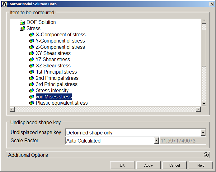
Figure 36. "von Mises stress".
Figure 37 represents the deformation of the truss and the stress distribution.
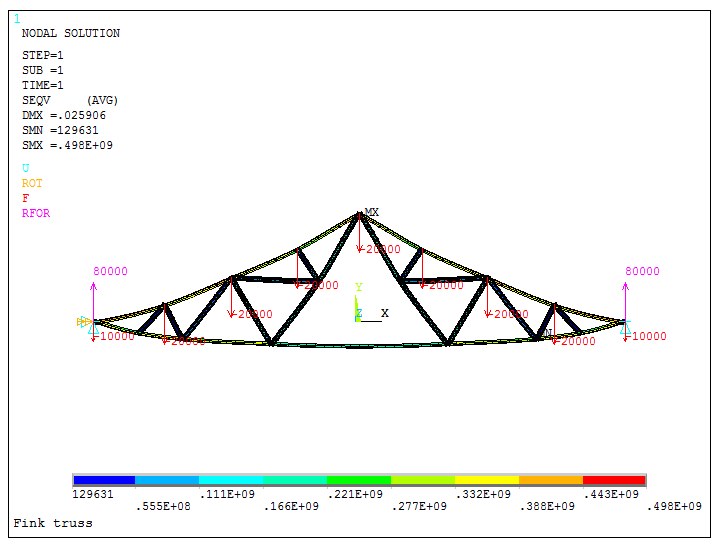
Figure 37. Deformation and stress distribution.