PROBLEM
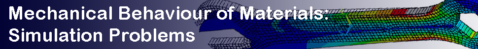
Figure 1 represents the structure for a container. The structure has three different types of sections: rectangular (80x40x2), L-shaped (L50x4) and Z-shaped (Z50x30x5) sections.
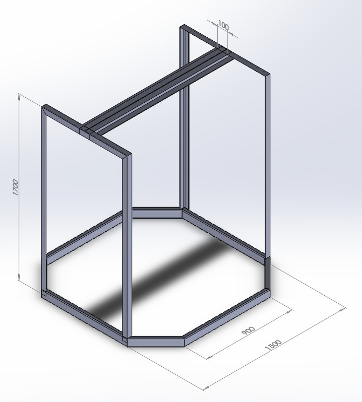
Figure 1. Container.
Table 1. Material properties.
| Steel | |
| Esteel | 210 GPa |
| Sy steel | 260 MPa |
| νsteel | 0.3 |
The maximum load acting on the container is 3000 N distributed on the basis. Calculate:
GEOMETRY OF THE MODEL
First, define a name for the problem. In this case "Container".
Utility Menu > File > Change Title
And define the problem type as "Structural":
Main Menu > Preferences > Structural
The element type used for this problem is "BEAM 3 node 189" (Figure 2):
Main Menu > Preprocessor > Element Type > Add/Edit/Delete
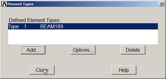
Figure 2. Element "BEAM 3 node 189".
Next, define the material properties for the steel:
Main Menu > Preprocessor > Material Props > Material Models
Input the data indicated in Table 1 (Figure 3).
Figure 3. Material Properties.
Next, define the three different sections for the model (Figure 4):
Main Menu > Preprocessor > Sections > Beam > Common Sections
They are defined as "HREC", "L" and "Z".
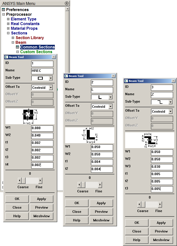
Figure 4. Defining the three sections.
Figures 5, 6 and 7 represent the geometric parameters of each section.
Main Menu > Preprocessor > Sections > Beam > Plot Section
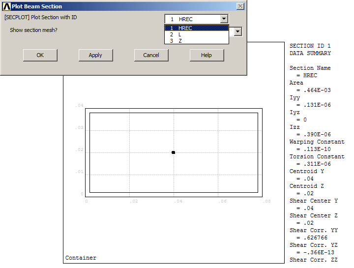
Figure 5. Rectangular section ("HREC").
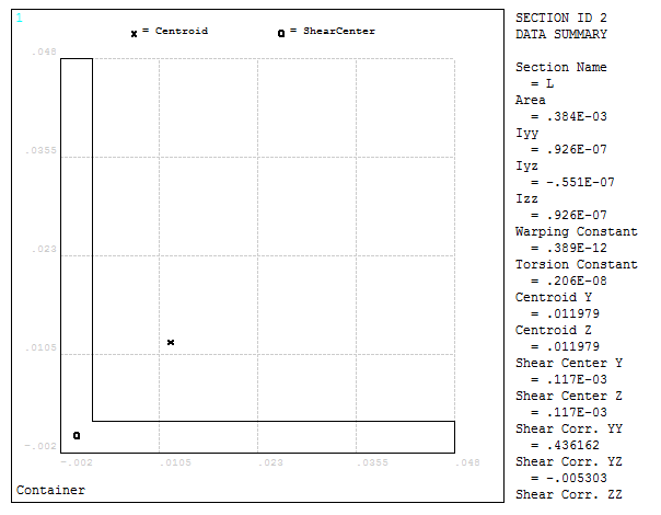
Figure 6. "L" section.
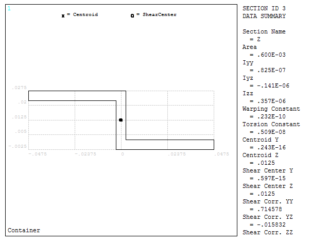
Figure 7. "Z" section.
Now, define the option "Z-axis up" so that the sections have the correct orientation for applying the loads.
Utility Menu > PlotCtrls > View Settings > Viewing Direction
The parameters are indicated in Figure 8.
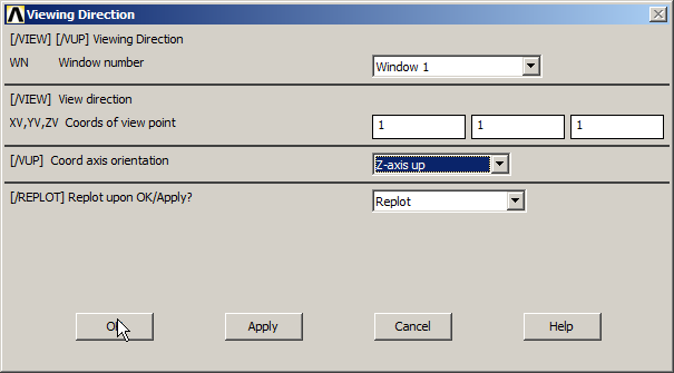
Figure 8. "Viewing Direction".
Now, as indicated in Table 2, input the coordinates for the 20 keypoints that define the structure of the container.
Main Menu > Preprocessor > Modeling > Create > Keypoints > In Active CS
Table 2. Coordinates of the 20 keypoints.
| Keypoint | X (m) | Y (m) | Z (m) |
| 1 | 0.45 | 0.75 | 0 |
| 2 | 0.75 | 0.45 | 0 |
| 3 | 0.75 | -0.45 | 0 |
| 4 | 0.45 | -0.75 | 0 |
| 5 | -0.45 | -0.75 | 0 |
| 6 | -0.75 | -0.45 | 0 |
| 7 | -0.75 | 0.45 | 0 |
| 8 | -0.45 | 0.75 | 0 |
| 9 | 0.75 | 0.45 | 1.7 |
| 10 | 0.75 | -0.45 | 1.7 |
| 11 | -0.75 | -0.45 | 1.7 |
| 12 | -0.75 | 0.45 | 1.7 |
| 13 | 0.75 | 0.05 | 1.7 |
| 14 | 0.75 | -0.05 | 1.7 |
| 15 | 0 | -0.05 | 1.7 |
| 16 | -0.75 | -0.05 | 1.7 |
| 17 | -0.75 | 0.05 | 1.7 |
| 18 | 0 | 0.05 | 1.7 |
| 19 | -0.75 | -0.05 | 2 |
| 20 | -0.75 | -0.05 | 2 |
Figure 9 represents the keypoints for the structure of the container.
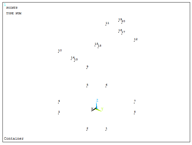
Figure 9. Keypoints for the container.
Create the lines to define the members:
Main Menu > Preprocessor > Modeling > Create > Lines > Lines > Straight Line
Table 3 indicates the order in which the lines are defined.
Table 3. Order to define the lines.
| Line | First keypoint | Second keypoint |
| 1 | 1 | 2 |
| 2 | 2 | 3 |
| 3 | 3 | 4 |
| 4 | 4 | 5 |
| 5 | 5 | 6 |
| 6 | 6 | 7 |
| 7 | 7 | 8 |
| 8 | 8 | 1 |
| 9 | 3 | 10 |
| 10 | 10 | 14 |
| 11 | 14 | 13 |
| 12 | 13 | 9 |
| 13 | 9 | 2 |
| 14 | 7 | 12 |
| 15 | 12 | 17 |
| 16 | 17 | 16 |
| 17 | 16 | 11 |
| 18 | 11 | 6 |
| 19 | 14 | 15 |
| 20 | 15 | 16 |
| 21 | 17 | 18 |
| 22 | 18 | 13 |
Figure 10 represents the structure with the lines numbered with option "Utility Menu – PlotCtrls – Numbering".
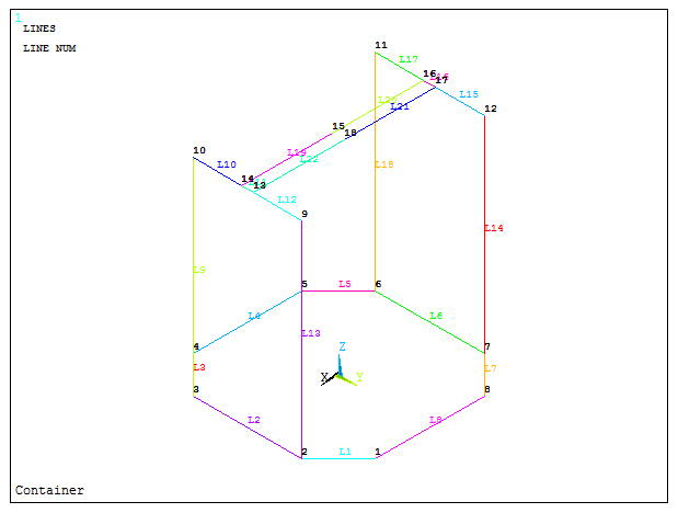
Figure 10. Structure of the container.
Now, each type of section has to be assigned to its corresponding line. Figures 11, 12 and 13 represent this process:
Main Menu > Preprocessor > Meshing > Mesh Attributes > Picked Lines
"HREC" section is for the lines at the bottom, "L" section is for the side lines and "Z" section is for the lines at the top.
For the correct orientation, select a previously defined keypoint or create one that is contained in the same plane in which the section has to be oriented. For this reason keypoints 19 and 20 have been created.
The sequence for generating the lines has the following criteria:
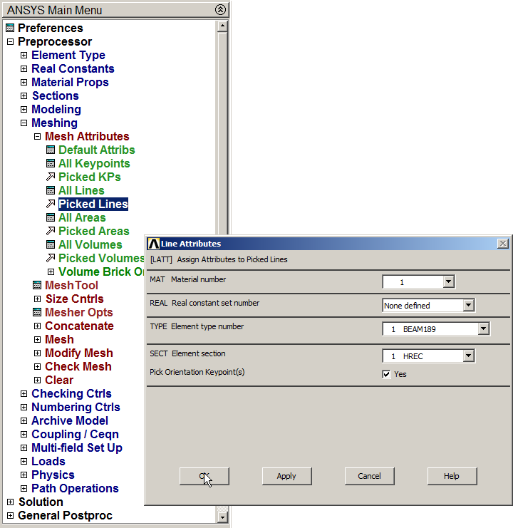
Figure 11. "Line Attributes" for "HREC" section.
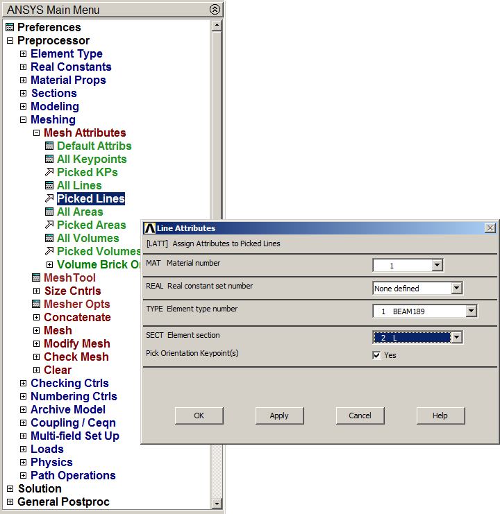
Figure 12. "Line Attributes for "L" section.
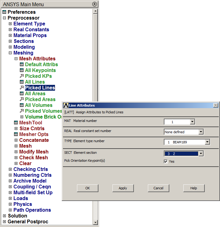
Figure 13. "Line Attributes" for "Z" section.
Next step is to define the element size for meshing the lines, that is 0.1 meters (Figure 14):
Main Menu > Preprocessor > Meshing > Size Cntrls > ManualSize > Lines > All Lines
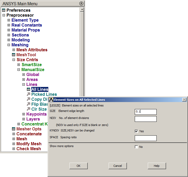
Figure 14. Defining the element size.
Finish the meshing process:
Main Menu > Preprocessor > Meshing > Mesh > Lines
And select "Pick All".
The structure can be represented as 3D model with the option "Size and Shape" (Figure 15).
Utility Menu > PlotCtrls > Style > Size and Shape
Activate "On" in "ESHAPE" option.
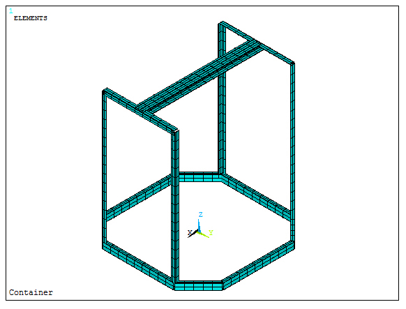
Figure 15. 3D model of the container.
LOADS AND BOUNDARY CONDITIONS
Since the 3000 N are distributed along the lines at the bottom, it is required to check the length of these lines:
Utility Menu > List > Picked Entities +
In the window "Model Query Picker" activate "Lines" in "On Entities" and then "Length" in "Query Item", as indicated in Figure 16.
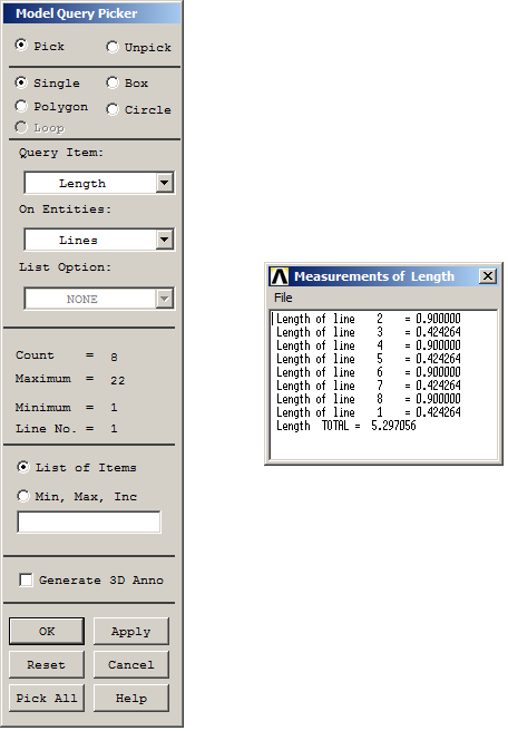
Figure 16. Length of the lines at the bottom.
Select these lines to apply the load (Figure 17):
Utility Menu > Select > Entities
Now, select "Lines", "By Location", "Z coordinate" and define "0" as the Z-coordinate where these lines are located.
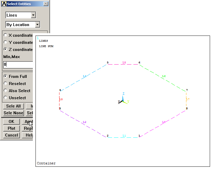
Figure 17. Select the lines at the bottom.
To apply the pressure on the members:
Utility Menu > Select > Entities
Select "Elements – Attached to" and activate "Lines" (Figure 18).
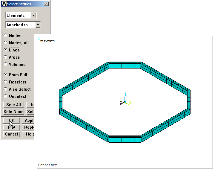
Figure 18. Select "Elements Attached to Lines".
Apply the pressure:
Main Menu > Preprocessor > Loads > Define Loads > Apply > Structural > Pressure > On Beams
Input the value for the distributed load along lines, that is 3000/5.297056, as indicated in Figure 19. Click "Pick All".
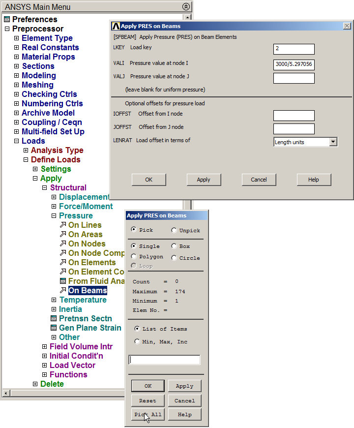
Figure 19. Applying pressure on beams.
Figure 20 represents the applied pressure on the selected lines.
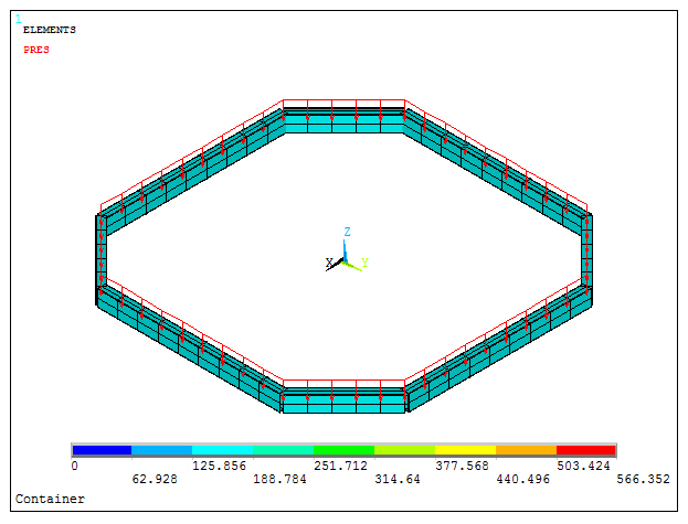
Figure 20. Applied pressure on beams.
Now, select all the geometric entities.
Utility Menu > Select > Everything
For the boundary conditions, keypoints 15 and 18 are considered the supporting points.
Main Menu > Preprocessor > Loads > Define Loads >Apply > Structural > Displacement > On Keypoints
Restrict displacements in directions "UX", "UY", "UZ" and rotation "ROTY" for keypoint 15 (Figure 21).
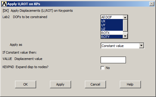
Figure 21. Boundary conditions for keypoint 15.
Figure 22 represents the boundary conditions for keypoint 18 (UX and UZ).
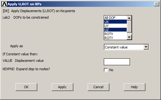
Figure 22. Boundary conditions for keypoint 18.
SOLUTION
Now, solve the problem:
Main Menu > Solution > Solve > Current LS
RESULTS
First, evaluate the deformation of the structure. As indicated in Figure 23, the maximum value is 0.011832 m:
Main Menu > General Postproc > Plot Results > Contour Plot > Nodal Solu
And select the option "Displacement vector sum" in "DOF Solution".
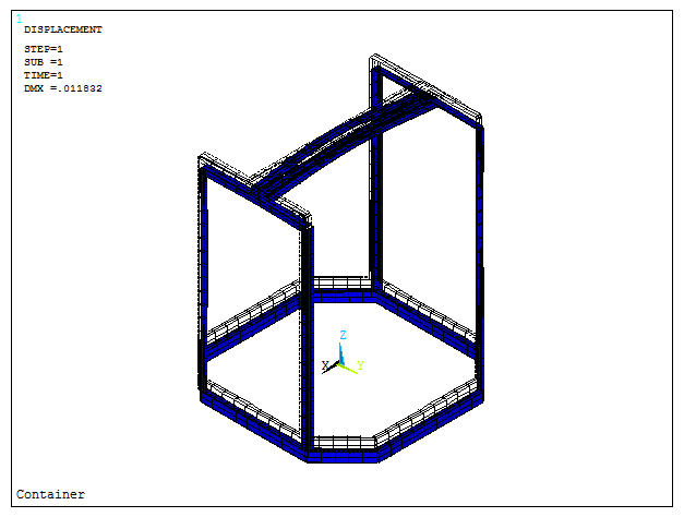
Figure 23. Deformation of the structure.
For the stress distribution in the structure:
Main Menu > General Postproc > Plot Results > Contour Plot > Nodal Solu
And select "von Mises stress" (Figure 24).
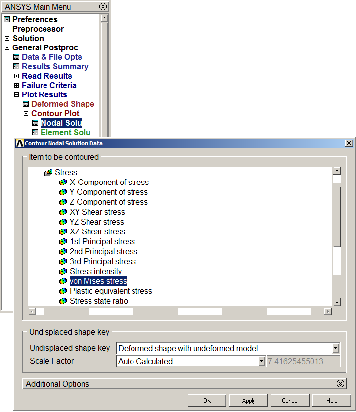
Figure 24. Stress distribution (Von Mises stress).
Figure 25 represents the stress distribution in the structure. The maximum value is 0.227·109 Pa.
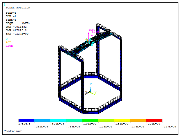
Figure 25. Structure with the stress distribution.
Finally, evaluate the stresses in every part of the structure: members at the bottom, side members and members at the top.
Figure 26 represents the stresses in the members at the bottom:
Utility Menu > Select > Entities
Select "Elements" and "By Attributes" with the option "Section ID num".
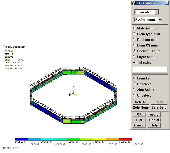
Figure 26. Stress distribution at the bottom.
In the same way, select the side members (Figure 27).
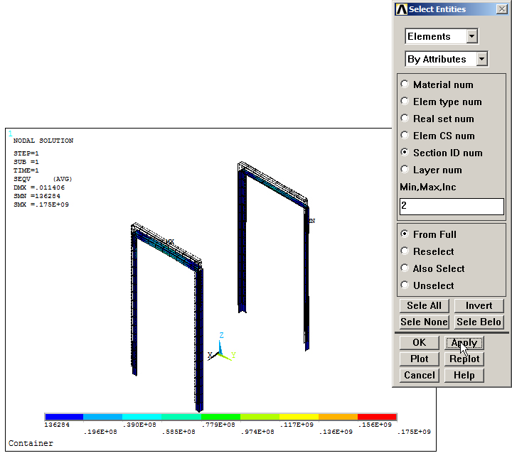
Figure 27. Stress distribution on side members.
And also the members at the top (Figure 28).
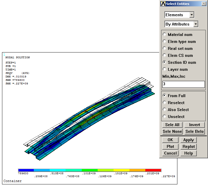
Figure 28. Stress distribution at the top.