PROBLEM
Figure 1 represents a 7 meter beam simply supported.
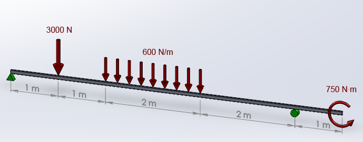
Figure 1. Beam simply supported.
The rectangular cross section has the dimensions 80 mm x 40 mm x 4 mm. Creation of file "80x40x4.sect" is required for the definition of this problem (see Customs sections).
Table 1 indicates the mechanical properties of the laminated steel for this beam.
Table 1. Mechanical properties.
| Laminated steel | |
| Esteel | 220 GPa |
| Sy steel | 275 MPa |
| νsteel | 0.292 |
Determine:
GEOMETRY OF THE MODEL
First of all, we define a name for the problem (Figure 2).
Utility Menu > File > Change Title
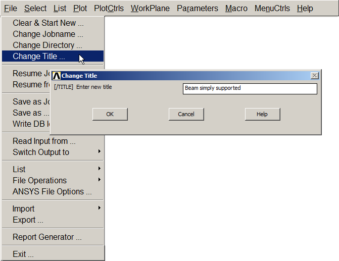
Figure 2. Change Title.
For this particular problem, change the axes orientation and define "Z-axis up" (Figure 3).
Utility Menu > PlotCtrls > View Settings > Viewing Direction
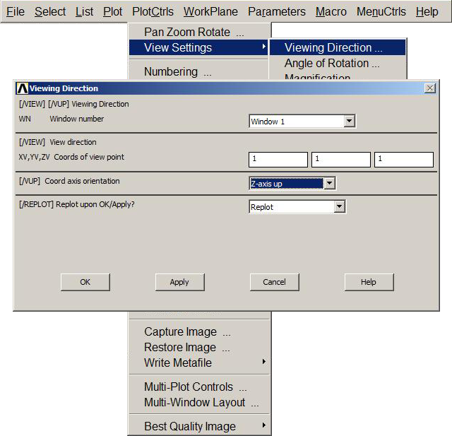
Figure 3. "Z-axis up".
Then, select the analysis type as "Structural" (Figure 4).
Main Menu > Preferences
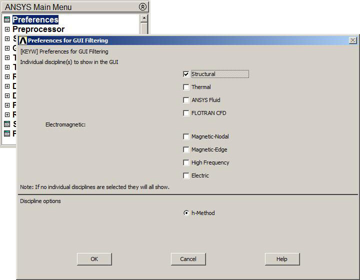
Figure 4. Structural analysis.
For this particular problem, the element type is "BEAM 188" (Figure 5).
Main Menu > Preprocessor > Element Type > Add/Edit/Delete
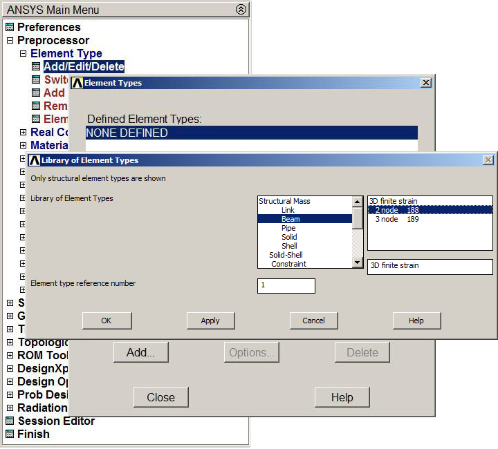
Figure 5. "BEAM 188" element.
Next, define the material properties (Figure 6).
Main Menu > Preprocessor > Material Props > Material Models
Select "Structural – Linear – Elastic – Isotropic" and define modulus of elasticity (EX) and Poisson's ratio (PRXY).
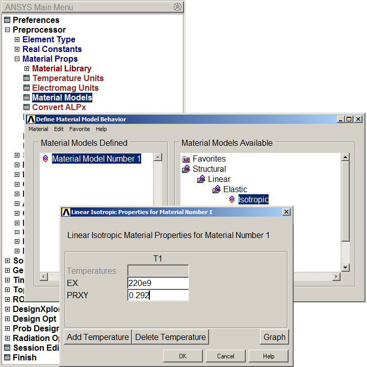
Figure 6. Mechanical properties for the laminated steel.
The cross section has to be defined previously (see Customs sections) and select "80x40x4" (Figure 7).
Main Menu > Preprocessor > Sections > Beam > Custom Sections > Read Sect Mesh
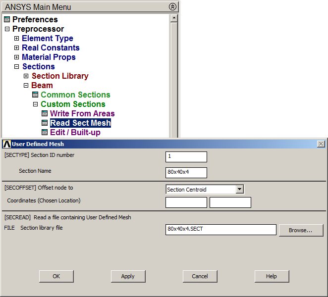
Figure 7. "Read Sect Mesh".
Table 2 indicates the coordinates for the keypoints.
Table 2. Keypoints coordinates.
| KEYPOINTS | X (m) | Y (m) | Z (m) |
| 1 | 0 | 0 | 0 |
| 2 | 0 | 1 | 0 |
| 3 | 0 | 2 | 0 |
| 4 | 0 | 4 | 0 |
| 5 | 0 | 6 | 0 |
| 6 | 0 | 7 | 0 |
Follow the instruction to create the keypoints (Figure 8):
Main Menu > Preprocessor > Modeling > Create > Keypoints > In Active CS
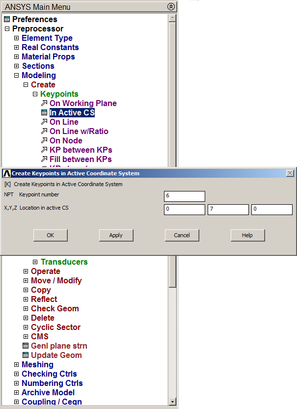
Figure 8. Create keypoints.
Figure 9 represents the graphic screen with the keypoints.
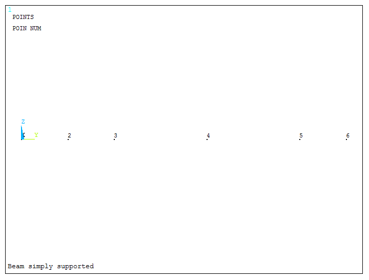
Figure 9. Graphic screen with the keypoints.
Next, create straight lines between the keypoints (Figure 10).
Main Menu > Preprocessor > Modeling > Create > Lines > Straight Line
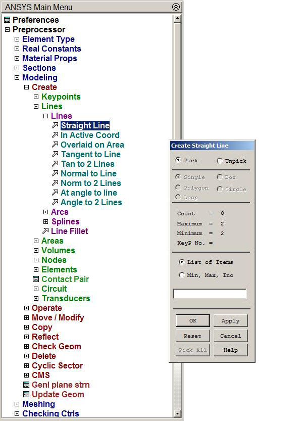
Figure 10. Create straight lines between keypoints.
Figure 11 represents the graphic screen with the lines that define the beam.
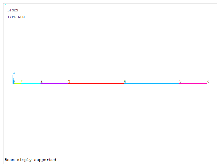
Figure 11. Graphic screen with the lines.
Next, mesh the beam (Figure 12):
Main Menu > Preprocessor > Meshing > Size Cntrls > ManualSize > Lines > Picked Lines
Select the lines and define the size element as 0.1 m.
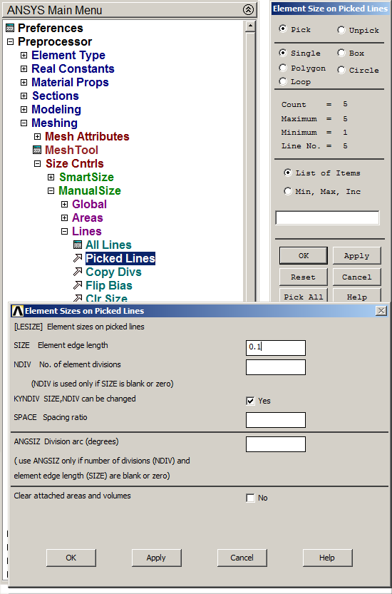
Figure 12. Meshing lines.
Finish the meshing process (Figure 13):
Main Menu > Preprocessor > Meshing > Mesh > Lines
And click "Pick All".
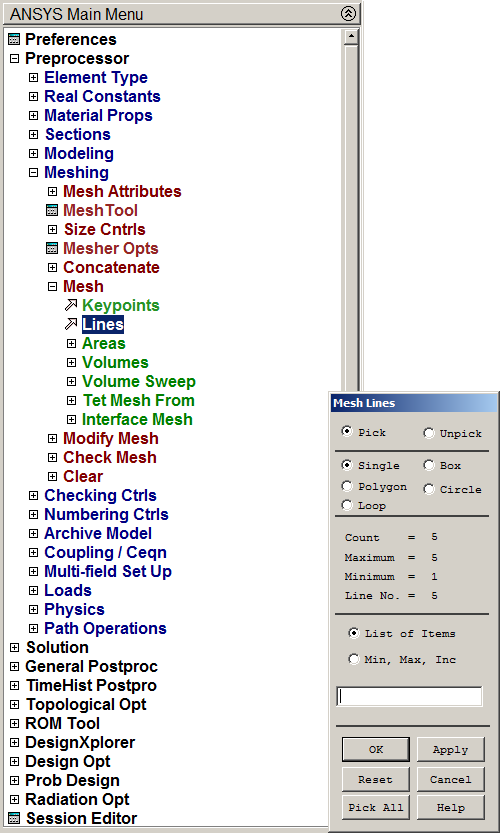
Figure 13. Mesh operation.
Figure 14 represents the model after the meshing process.
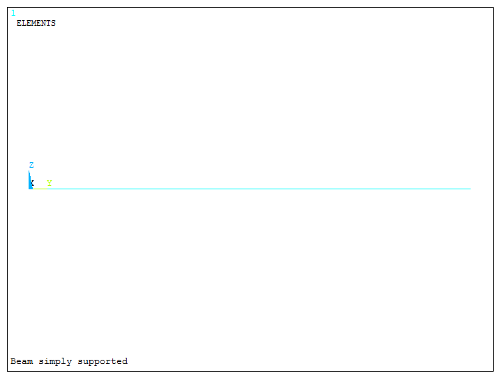
Figure 14. Meshed beam.
LOADS AND BOUNDARY CONDITIONS
For the boundary conditions, the left end of the beam is pinned (Figure 15).
Main Menu > Preprocessor > Loads > Define Loads > Apply > Structural > Displacement > On Keypoints
Select the left keypoint and click on UX, UY, UZ and ROTY.
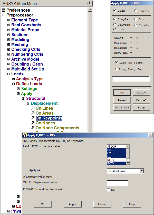
Figure 15. Restriction at left end of the beam.
At simply support location, restrict displacements in UX and UZ directions (Figure 16).
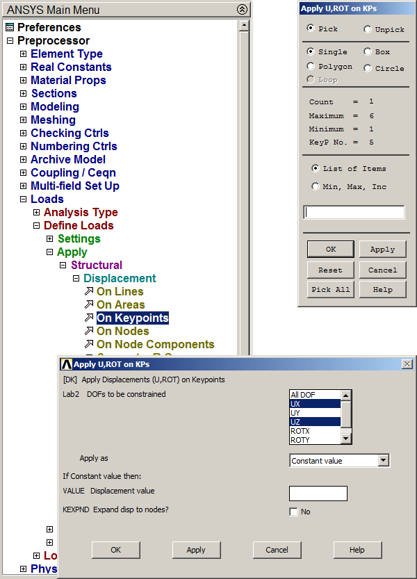
Figure 16. Restrictions at simply support location.
After that, apply forces acting on the beam. First, the concentrated load of 3000 N (Figure 17):
Main Menu > Preprocessor > Loads > Define Loads > Apply > Structural > Force/Moment > On Nodes
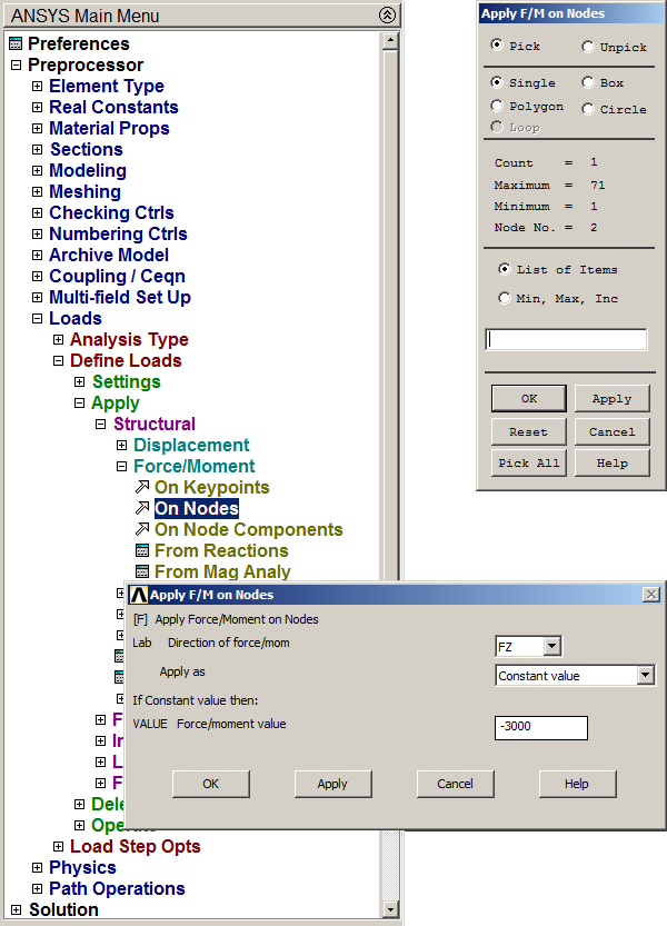
Figure 17. Concentrated load of 3000 N.
Apply the moment at the right end of the beam (Figure 18).
Main Menu > Preprocessor > Loads > Define Loads > Apply > Structural > Force/Moment > On Nodes

Figure 18. Bending moment at right end.
Next, define the distributed load of 600 N/m. Since this load acts along 2 meters and on 21 nodes, for each node there is a concentrated force of (600x2)/21, that is, 57,14 N per node.
Select the particular nodes where this load acts:
Utility Menu > Select > Entities
As indicated in Figure 19, define the range Y = [2, 4].
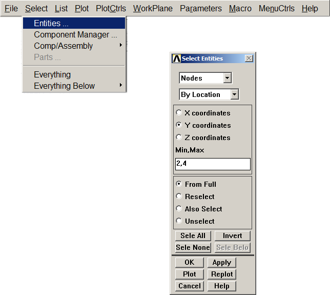
Figure 19. Select the range for the distributed load.
Click "Pick All" and define the value for the load (Figure 20).
Main Menu > Preprocessor > Loads > Define Loads > Apply > Structural > Force/Moment > On Nodes

Figure 20. Value for the distributed load.
Finally, select all the geometric entities:
Utility Menu > Select > Everything
SOLUTION
Next step is to solve the problem (Figure 21):
Main Menu > Solution > Solve > Current LS
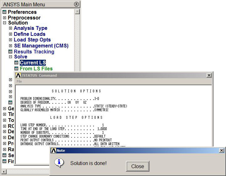
Figure 21. Solution.
RESULTS
Analyze the results. First, obtain the external reactions.
Main Menu > General Postproc > List Results > Reaction Solu
Select "All items" in the "List Reaction Solution" window.
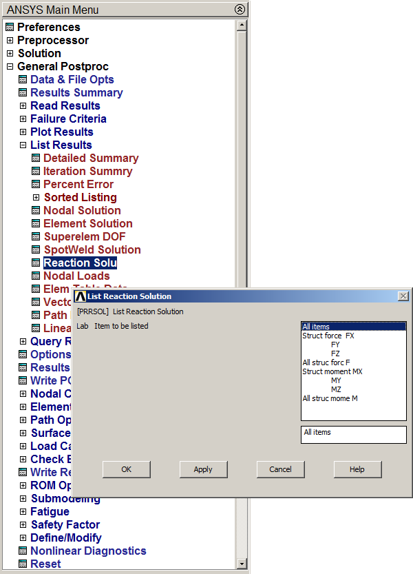
Figure 22. Reaction Solu.
The values of the external reactions are listed in Figure 23.
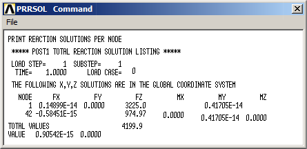
Figure 23. List of the external reactions.
For the deformation of the beam (Figure 24):
Main Menu > General Postproc > Plot Results > Deformed Shape
And select the option "Def+undef edge".
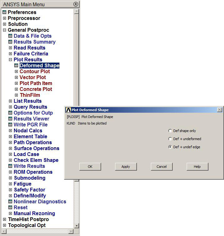
Figure 24. Deformation of the beam.
Figure 25 represents the deformation of the beam with the maximum value (DMX).
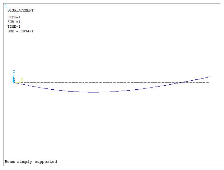
Figure 25. Deformation of the beam.
To analyze the shear forces and bending moments acting on the beam, define the labels "SHEARi", "SHEARj", "MOMi", "MOMj" and the corresponding items for the required results: SMISC, NMISC, … (ANSYS HELP).
Figure 26 represents the definition of the label "SHEARi" for the shear forces:
Main Menu > General Postproc > Element Table > Define Table
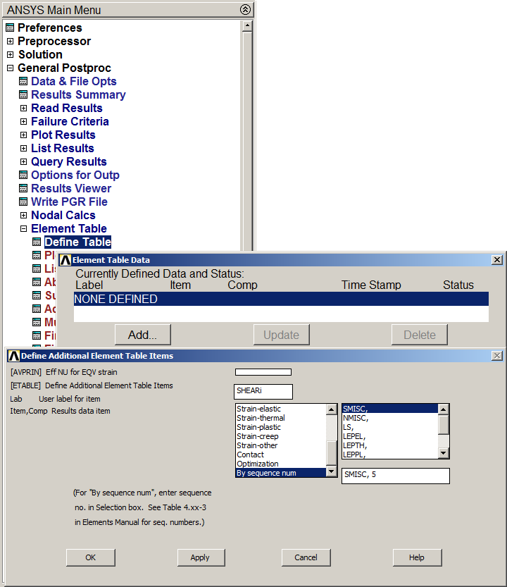
Figure 26. Define Table.
Figure 27 shows the list with the four defined labels.
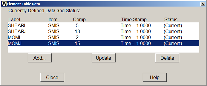
Figure 27. Element Table Data.
Represent the distribution of the shear forces (Figure 28):
Main Menu > General Postproc > Plot Results > Contour Plot > Line Elem Res
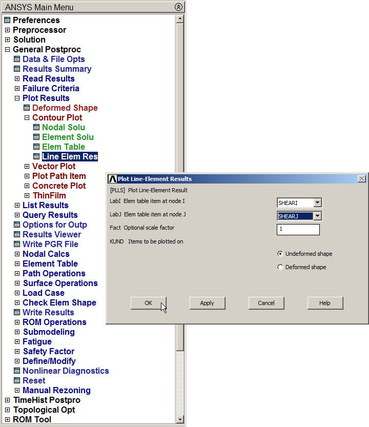
Figure 28. Select labels for shear forces.
The distribution of shear forces on the beam are represented in Figure 29.
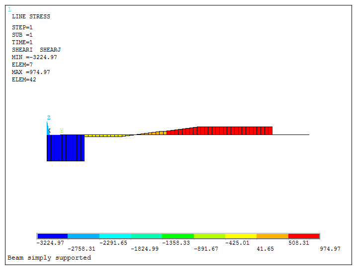
Figure 29. Shear forces.
Finally, select the labels for the bending moments (Figure 30):
Main Menu > General Postproc > Plot Results > Contour Plot > Line Elem Res

Figure 30. Selecting bending moments labels.
Figure 31 represents the bending moments on the beam.
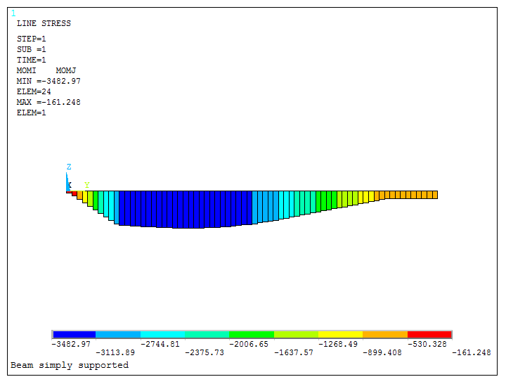
Figure 31. Bending Moments.