
PROBLEM
Figure 1 shows a polypropylene (PP) bracket. A distributed pressure acts in the third quadrant of the circular hole varying from 0 to pmax and in the fourth quadrant varying from pmax to 0. For F=100 N:
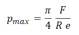
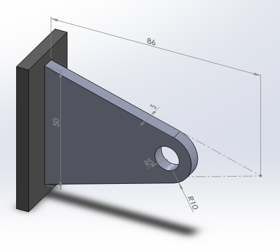
Figure 1. Plastic bracket.
Determine the stress distribution and the minimum value of the thickness, so that the material works in the elastic field without plastic deformation.
Table 1. Material properties.
| Polypropylene | |
| Epolypropylene | 1200 N/mm2 |
| Sy polypropylene | 45 N/mm2 |
| νpolypropylene | 0.43 |
GEOMETRY OF THE MODEL
First of all, define a name for the problem: "Plastic bracket":
Utility Menu > File > Change Title
And select the option "Structural":
Main Menu > Preferences > Structural
In this case, define some scalar parameters (Figure 2):
Utility Menu > Parameters > Scalar Parameters
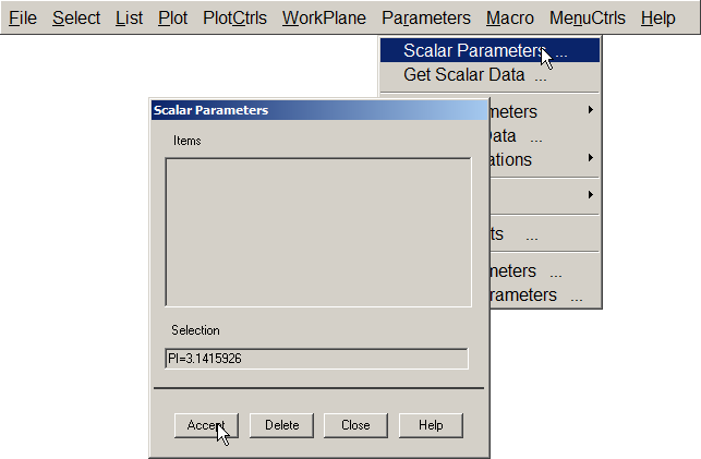
Figure 2. Scalar Parameters.
In the same way, input the values for the applied force (F=100 N), "pi" number (PI=3.1415926), the radius for the hole (R=0.005 m) and the thickness (E=0.005 m), as indicated in Figure 3.
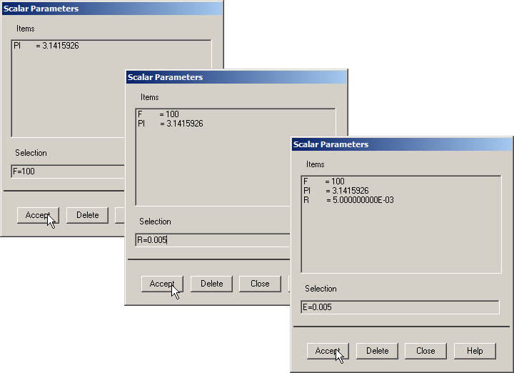
Figure 3. Definition of some scalar parameters.
Next, define the element type:
Main Menu > Preprocessor > Element Type > Add/Edit/Delete
Select the element "Solid Plane 8 node 183" (Figure 4).
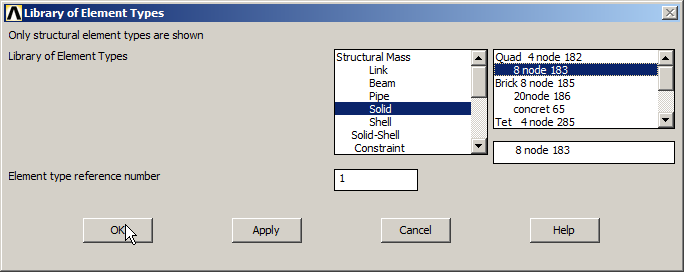
Figure 4. Element "Solid Plane 8 node 183".
Then, in "Options" select "Plane strs w/thk" to define the thickness (Figure 5).
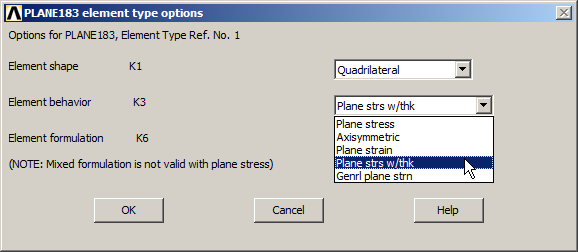
Figure 5. "Plane strs with thickness".
Input "E" as the value for the thickness in "Real Constants" (Figure 6):
Main Menu > Preprocessor > Real Constants > Add/Edit/Delete
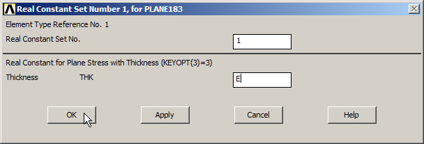
Figure 6. Thickness of 5 mm ("E").
Now, define the mechanical properties for the polypropylene:
Main Menu > Preprocessor > Material Props > Materials Models
Input the values for the material as indicated in Figure 7:
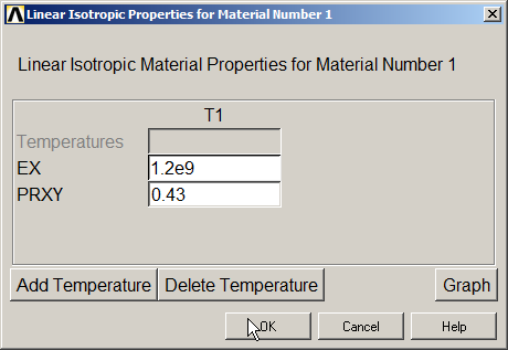
Figure 7. Mechanical properties for the polypropylene.
For the geometry, create the three keypoints indicated in Table 2.
Table 2. Keypoint coordinates.
| Keypoint | X (m) | Y (m) | Z (m) |
| 1 | 0 | -0.025 | 0 |
| 2 | 0 | 0.025 | 0 |
| 3 | 0.086 | 0 | 0 |
Main Menu > Preprocessor > Modeling > Create > Keypoints > In Active CS
Figure 8 represents the process to create these keypoints.
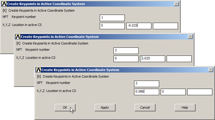
Figure 8. Creating the three keypoints.
Figure 9 shows the graphic screen with the created keypoints.
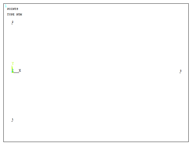
Figure 9. Graphic screen with the three keypoints.
After that, create the lines, as indicated in Figure 10:
Main Menu > Preprocessor > Modeling > Create > Lines > Straight Line

Figure 10. Graphic screen with the lines.
Now, define the radius of curvature with the option "Line Fillet":
Main Menu > Preprocessor > Modeling > Create > Lines > Line Fillet
Select the two lines and input the value of 0.01m for the radius (Figure 11):
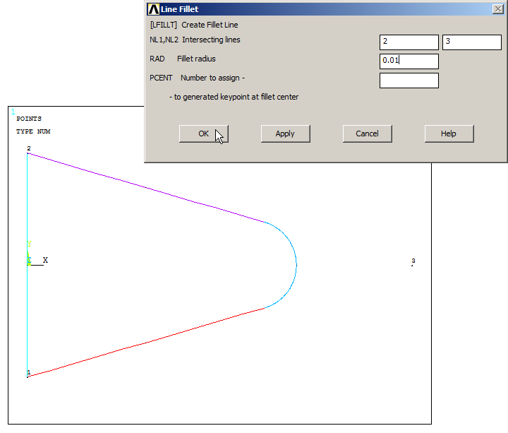
Figure 11. Radius of curvature with "Line Fillet" option.
Now, create the area (Figure 12):
Main Menu > Preprocessor > Modeling > Create > Areas > Arbitrary > By Lines
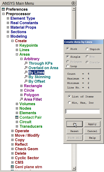
Figure 12. Creating the area.
Create the circular area for the hole:
Main Menu > Preprocessor > Modeling > Create > Areas > Circle > Solid Circle
Input the parameters indicated in Figure 13 for this circular area.
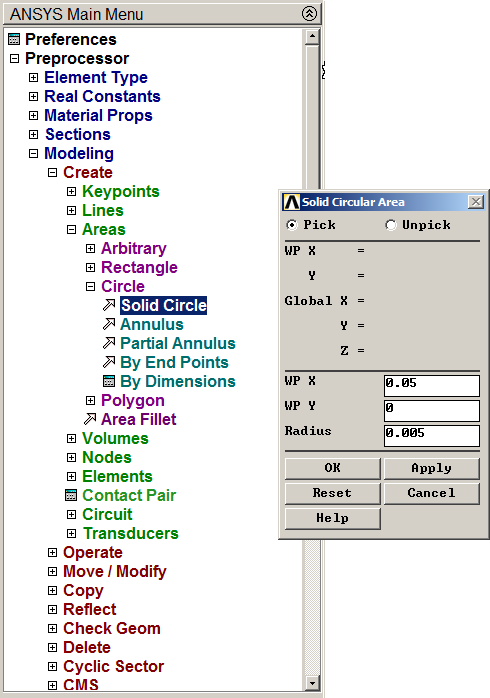
Figure 13. Circular area for the hole.
Activate the "Numbering" option for areas:
Utility Menu > PlotCtrls > Numbering
Click "On" in "Area numbers".
Figure 14 represents the two areas for the model.

Figure 14. The two areas for the model.
Next step is to subtract the circular area:
Main Menu > Preprocessor > Modeling > Operate > Booleans > Subtract > Areas
Select all areas, "OK" and then select the circular area and "OK". Figure 15 represents the model.
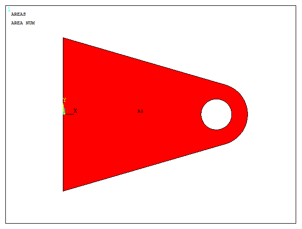
Figure 15. Plastic bracket after "Subtract" operation.
Now, define the element size for the mesh. The element size is 0.001 m, as indicated in Figure 16:
Main Menu > Preprocessor > Meshing > Size Cntrls > ManualSize > Areas > All Areas
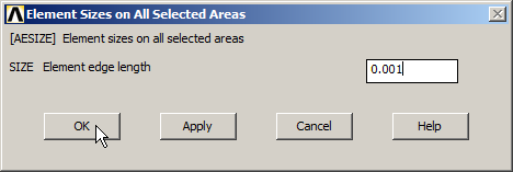
Figure 16. Element size for meshing.
To finish the meshing process:
Main Menu > Preprocessor > Meshing > Mesh > Areas > Free
Figure 17 represents the meshed model.
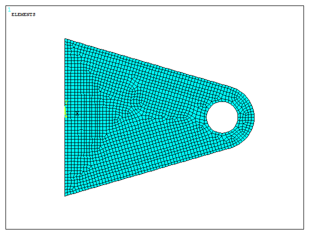
Figure 17. Meshed model.
LOADS AND BOUNDARY CONDITIONS
For the boundary conditions, the bracket is fixed at the left side. Apply the restriction "All DOF" (All Degrees of Freedom) to the line on the left:
Main Menu > Preprocessor > Loads > Define Loads > Apply > Structural > Displacement > On Lines
Select the line on the left.
Next, define the pressure that is distributed on the thickness:
Main Menu > Preprocessor > Loads > Define Loads > Apply > Structural > Pressure > On Lines
In the third quadrant of the circular hole, apply the pressure as indicated in Figure 18.
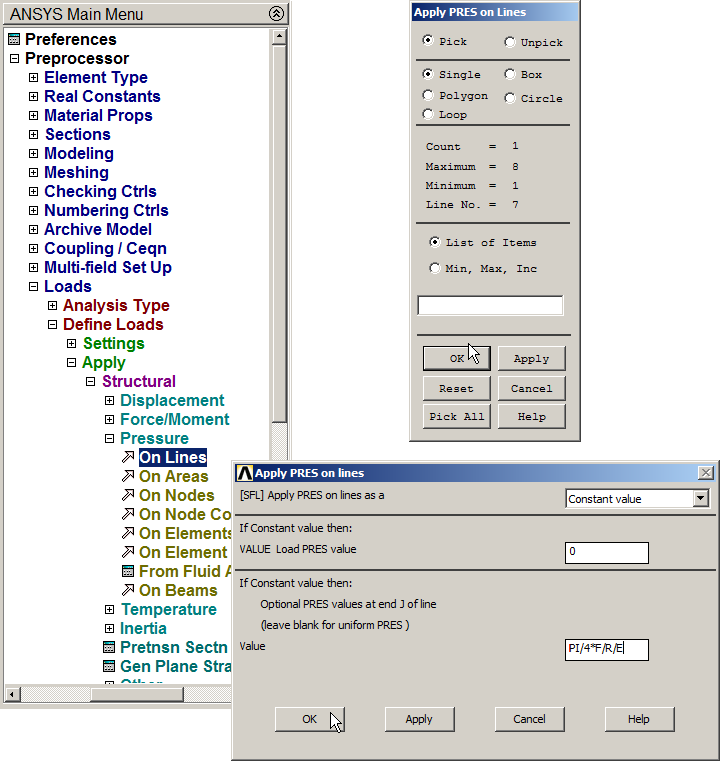
Figure 18. Applying the pressure in the third quadrant of the circular hole.
In the same way, apply the same pressure at the other side of the circular hole, that is the fourth quadrant as indicated in Figure 19.
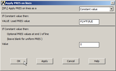
Figure 19. Applying the pressure in the fourth quadrant of the circular hole.
Use the option "Symbols" to represent the model:
Utility Menu > PlotCtrls > Symbols
And activate "Pressures" in "Surface Load Symbols" and "Arrows" in "Show pres and convect as". Figure 20 represents the graphic screen of the model with the boundary conditions and the applied pressure.
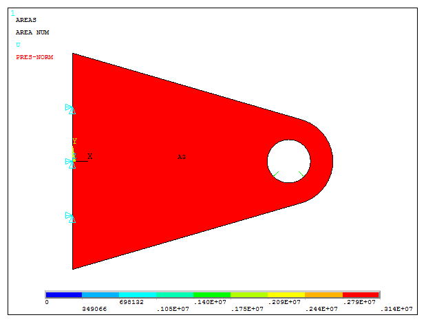
Figure 20. Model with the boundary conditions and the applied pressure.
SOLUTION
Solve the problem.
Main Menu > Solution > Solve > Current LS
Click "OK".
RESULTS
First, list the reactions (Figure 21):
Main Menu > General Postproc > List Results > Reaction Solu
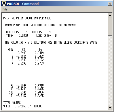
Figure 21. Reactions on the nodes.
For the stress distribution on the bracket (Figure 22):
Main Menu > General Postproc > Plot Results > Contour Plot > Nodal Solu
And select "Stress – von Mises stress".
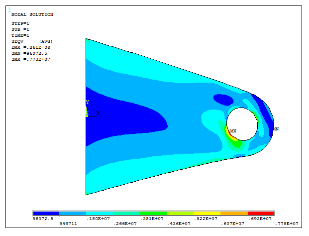
Figure 22. Stress distribution.
To optimize the thickness for this particular model, take into account the relation between the value of the maximum stress and the yield stress multiplied by the initial thickness, as indicated in Figure 23. The new value for the thickness is 8.6533·10-4 m.
Utility Menu > Parameters > Scalar Parameters
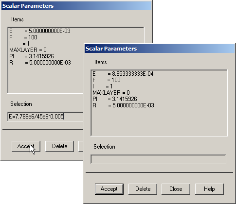
Figure 23. Optimizing the thickness.
Define again the "Real Constants", as indicated in Figure 24:
Main Menu > Preprocessor > Real Constants > Add/Edit/Delete
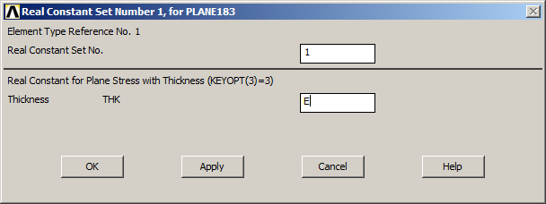
Figure 24. New thickness in "Real Constants".
Finally, solve the problem and represent the stress distribution (Figure 25).
Main Menu > General Postproc > Plot Results > Contour Plot > Nodal Solu
Select "Stress – von Mises stress".
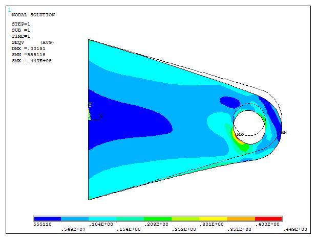
Figure 25. Stress distribution for the new thickness.