
PROBLEM
Figure 1 shows a wrench made of a nickel alloy steel.
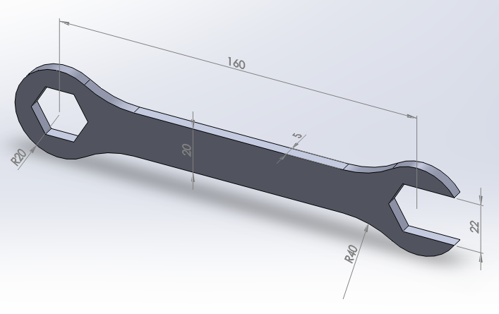
Figure 1. Wrench.
A force of 1000 N acts on the hand support when the wrench is working by setting a screw.
Calculate the maximum equivalent stress and the maximum deformation. Table 1 shows the mechanical properties of this nickel alloy steel.
Table 1. Material properties.
| Nickel alloy steel | |
| Enickel alloy steel | 207 GPa |
| νnickel alloy steel | 0.3 |
GEOMETRY OF THE MODEL
First of all, define the type of analysis, that is "Structural".
Main Menu > Preferences > Structural
For this particular problem, the element type is "Solid 8 node 183" (Figure 2).
Main Menu > Preprocessor > Element Type > Add/Edit/Delete
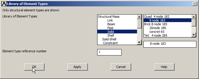
Figure 2. Element "Solid 8 node 183".
In "Options", select "Plane strs w/thk" to define the thickness of the model, as indicated in Figure 3.
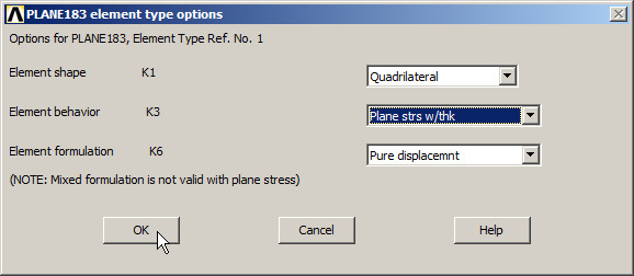
Figure 3. Plane stress with thickness.
Input the thickness in "Real Constants" (Figure 4):
Main Menu > Preprocessor > Real Constants > Add/Edit/Delete

Figure 4. Thickness (5 mm).
Now define the material properties (Figure 5):
Main Menu > Preprocessor > Material Props > Material Models
Define the material as "Structural – Linear – Elastic – Isotropic".
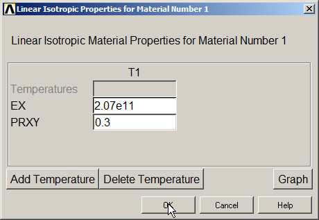
Figure 5. Material properties.
For the geometric model, create a grid in the working plane (Figure 6):
Utility Menu > WorkPlane > Display Working Plane
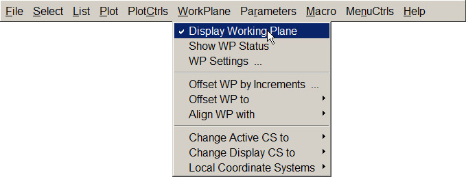
Figure 6. "Display Working Plane".
Select "WP Settings" (Figure 7):
Utility Menu > WorkPlane > WP Settings …
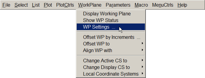
Figure 7. "WP Settings".
The parameters that define the grid are displayed in Figure 8.
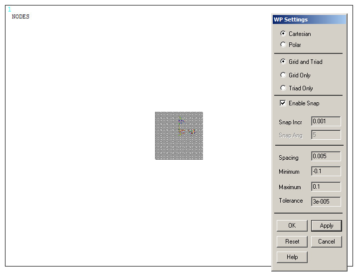
Figure 8. Parameters for the grid.
Figure 9 shows the generated grid and the "Pan-Zoom-Rotate" tool from the "Utility Menu – PlotCtrls" to set the views.
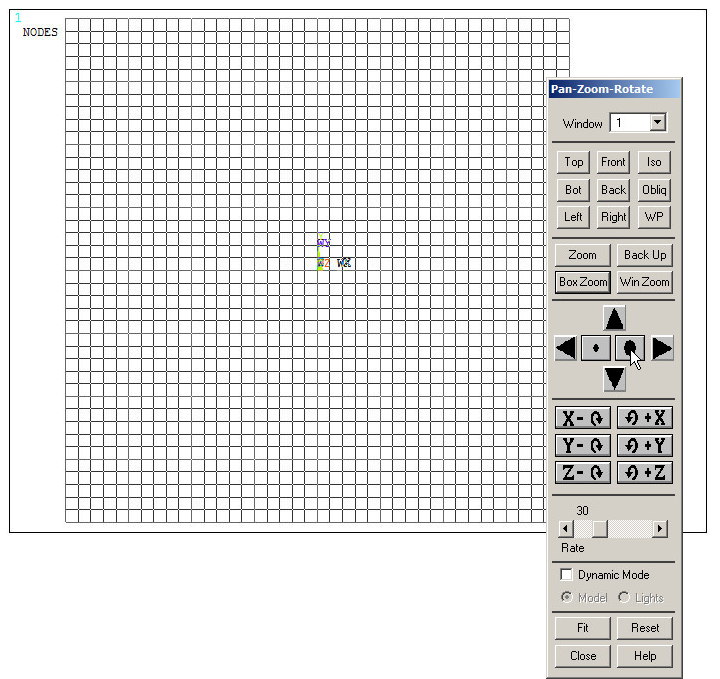
Figure 9. "Pan-Zoom-Rotate" option.
Now, create a rectangular area with the geometric characteristics indicated in Figure 10.
Main Menu > Preprocessor > Modeling > Create > Areas > Rectangle > By 2 Corners
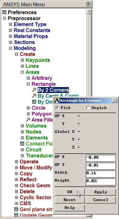
Figure 10. Creating a rectangular area.
Figure 11 displays graphically the rectangular area for the model.
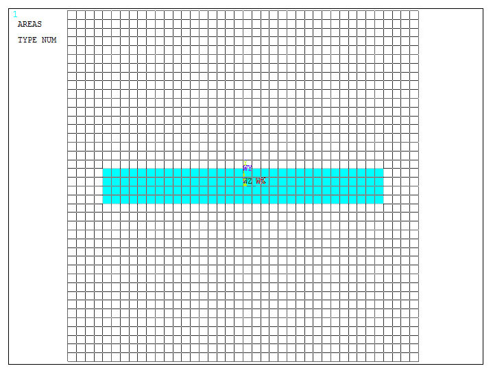
Figure 11. Rectangular area for the model.
Then create two circular areas as indicated in Figure 12.
Main Menu > Preprocessor > Modeling > Create > Areas > Circle > Solid Circle
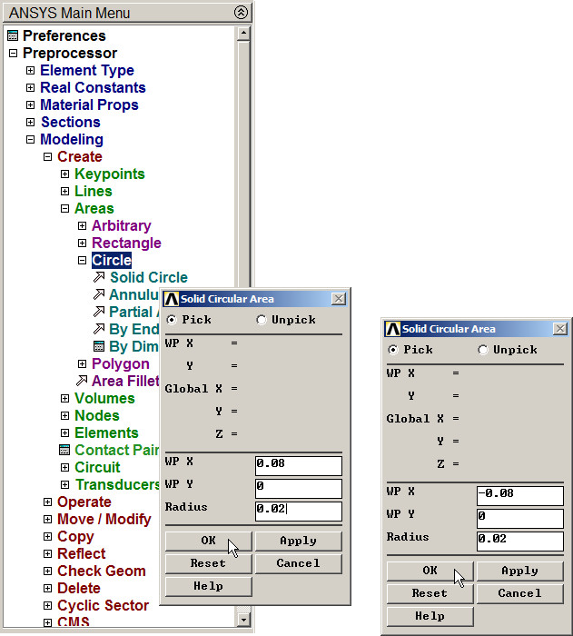
Figure 12. Creating two circular areas.
Figure 13 shows the three areas for the model.
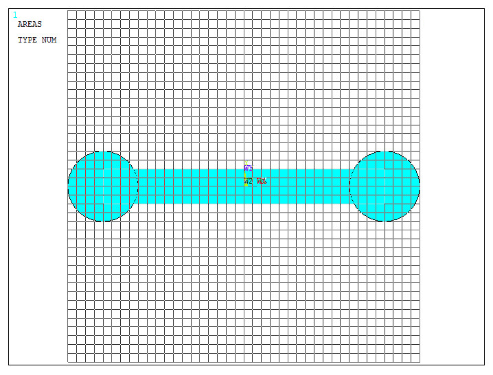
Figure 13. Created areas with the grid.
Now, "Add" areas (Figure 14):
Main Menu > Preprocessor > Modeling > Operate > Booleans > Add > Areas
Select the three areas and "OK".
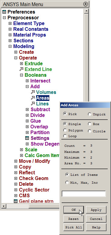
Figure 14. "Add Areas".
The three added areas are displayed graphically in Figure 15.
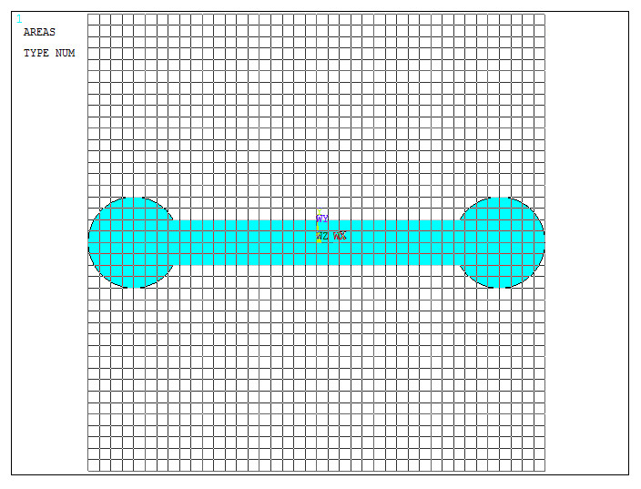
Figure 15. Model after "Add Areas" operation.
Now create the hexagonal area:
Main Menu > Preprocessor > Modeling > Create > Areas > Polygon > By Inscribed Rad
Define the number of sides and the inscribed radius as indicated in Figure 16.
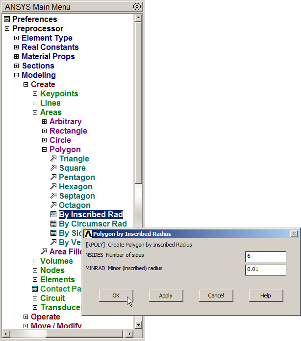
Figure 16. Hexagonal area.
This hexagonal area has to be moved to the right end (Figure 17):
Main Menu > Preprocessor > Modeling > Move/Modify > Areas
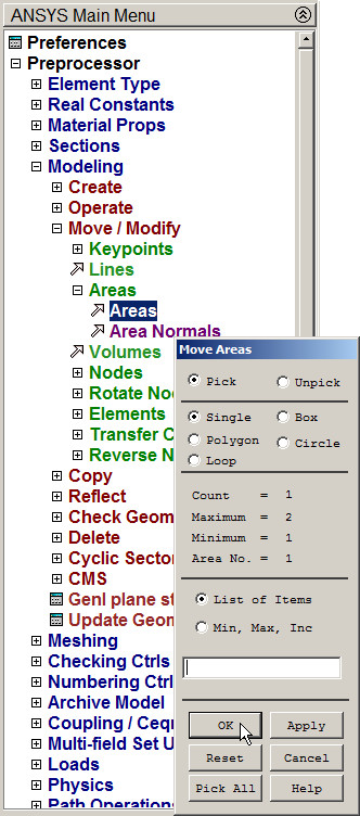
Figure 17. Moving the hexagonal area.
Select the hexagonal area (Figure 18).
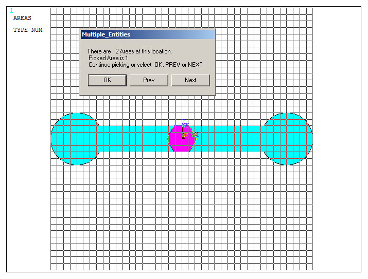
Figure 18. Selecting the hexagonal area.
And define the direction and distance for the "Move" operation (Figure 19).
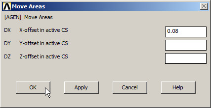
Figure 19. Moving the area 80 mm.
Figure 20 shows the plotted model from "Utility Menu – Plot – Replot".
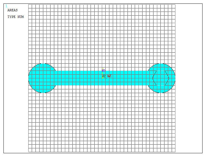
Figure 20. "Replot" the model.
For the left side, copy the hexagonal area, as indicated in Figure 21.
Main Menu > Preprocessor > Modeling > Copy > Areas
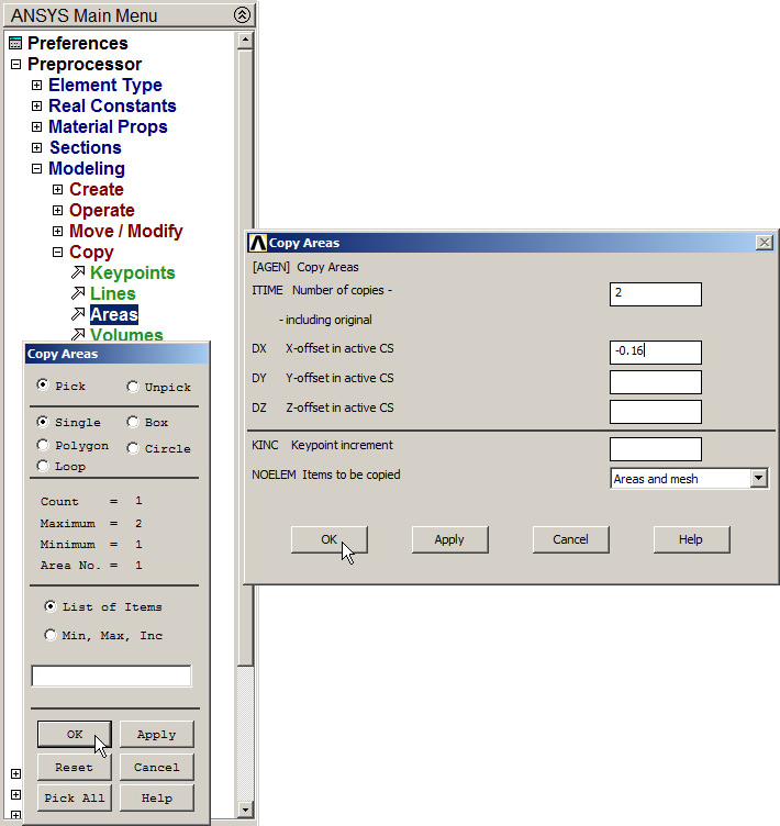
Figure 21. Copying the hexagonal area.
Use "Pan-Zoom-Rotate" tool to display the right end of the model, as indicated in Figure 22.
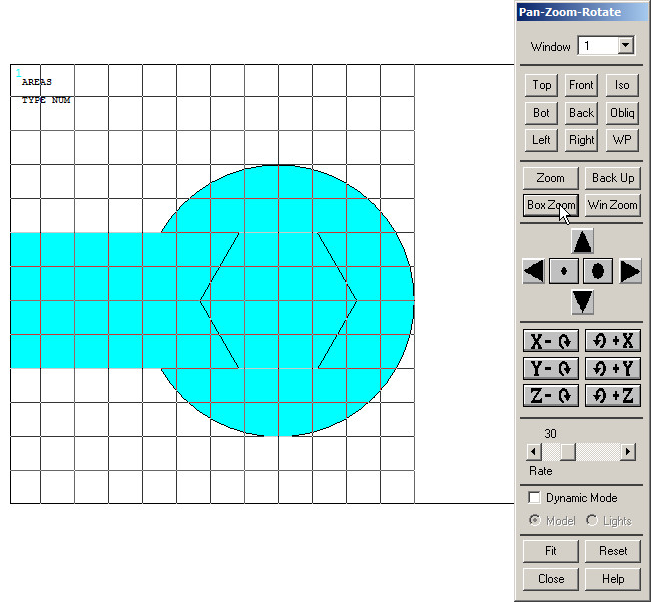
Figure 22. Zoom of the right end.
For the geometry of this part of the model, create two new keypoints:
Main Menu > Preprocessor > Modeling > Create > Keypoints > On Working Plane
Click and drag the cursor on the working plane to define the two keypoints, as indicated in Figure 23.
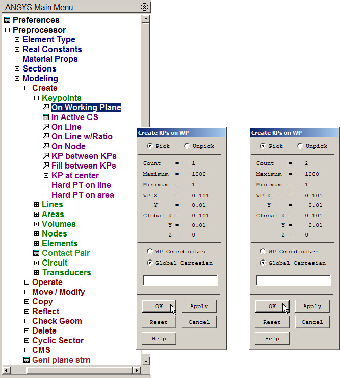
Figure 23. Creating Keypoints.
Figure 24 shows the new keypoints.
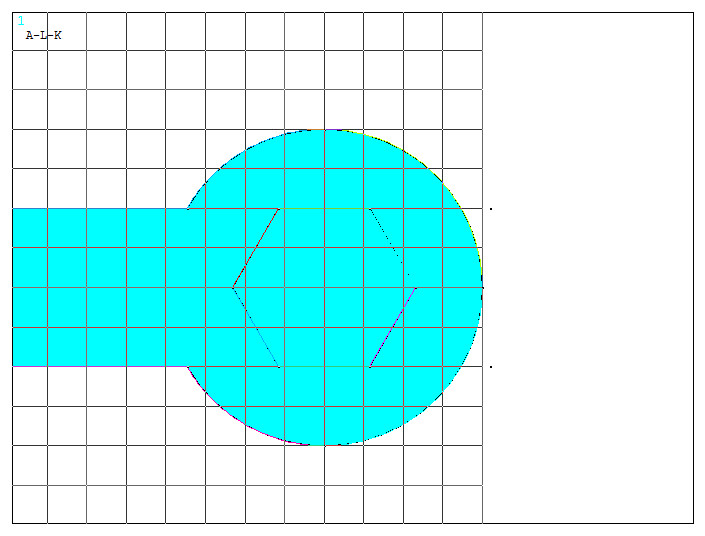
Figure 24. Created Keypoints.
Now, create a new area through the 5 keypoints indicated in Figure 25.
Main Menu > Preprocessor > Modeling > Create > Areas > Arbitrary > Through KPs
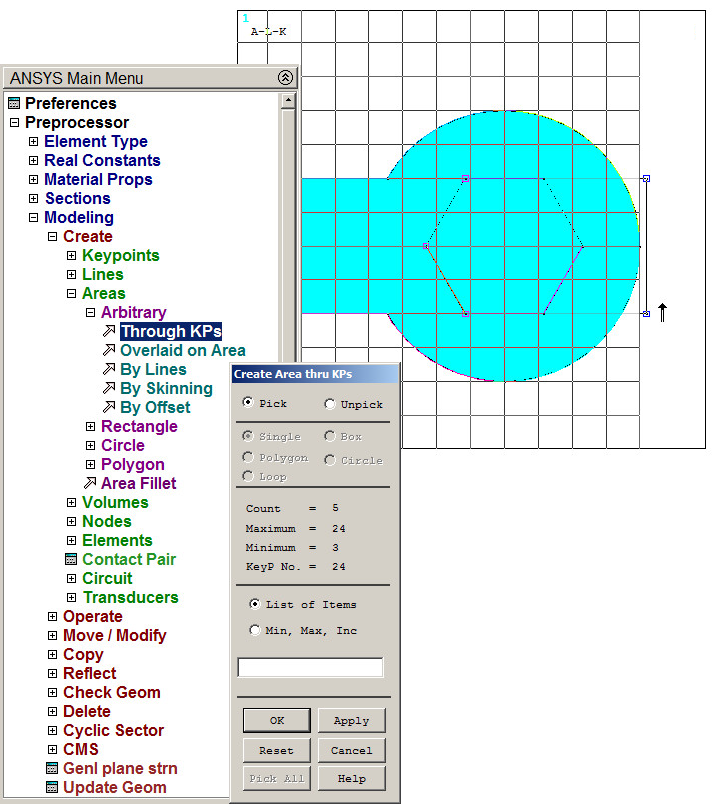
Figure 25. Creating a new area through keypoints.
The new area is overlapped with the hexagonal area. So, the latter must be removed (Figure 26):
Main Menu > Preprocessor > Modeling > Delete > Area and Below
The option "Delete Area and Below" removes all the geometric entities attached to the area.
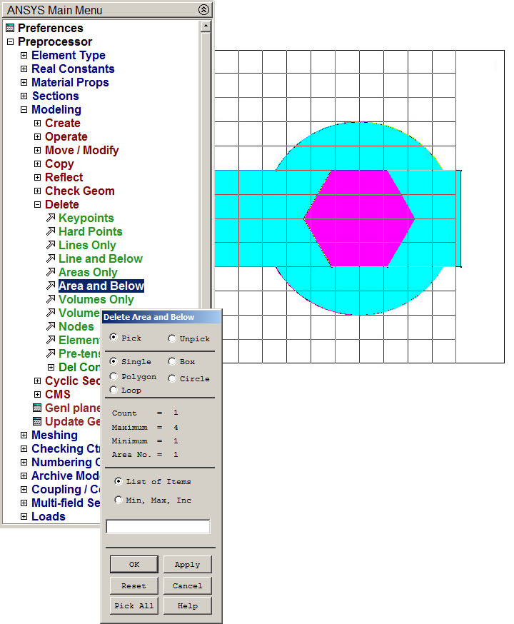
Figure 26. Delete the hexagonal area.
Number the areas (Figure 27):
Utility Menu > PlotCtrls > Numbering
Activate "AREA".
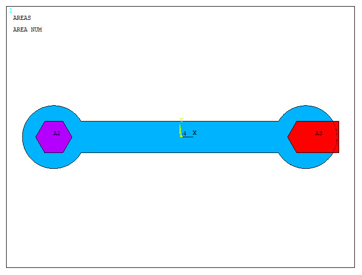
Figure 27. Numbering areas.
Now, subtract the two areas located at the two sides of the model.
Main Menu > Preprocessor > Modeling > Operate > Booleans > Subtract > Areas
First, select all the areas, click "OK". Then, select the two areas to be subtracted and "OK". Figure 28 represents the model after "Subtract" operation.
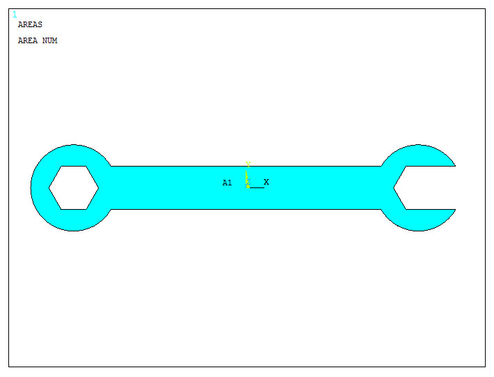
Figure 28. Model after "subtract" operation.
Activate "Multi-Plots" option to display the geometry of the model (Figure 29).
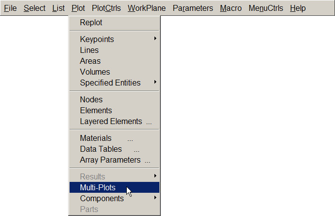
Figure 29. "Multi-Plots" option.
Number all areas and lines. Figure 30 displays graphically the model for the wrench.
Utility Menu > PlotCtrls > Numbering
And activate the options "Line numbers" and "Area numbers".
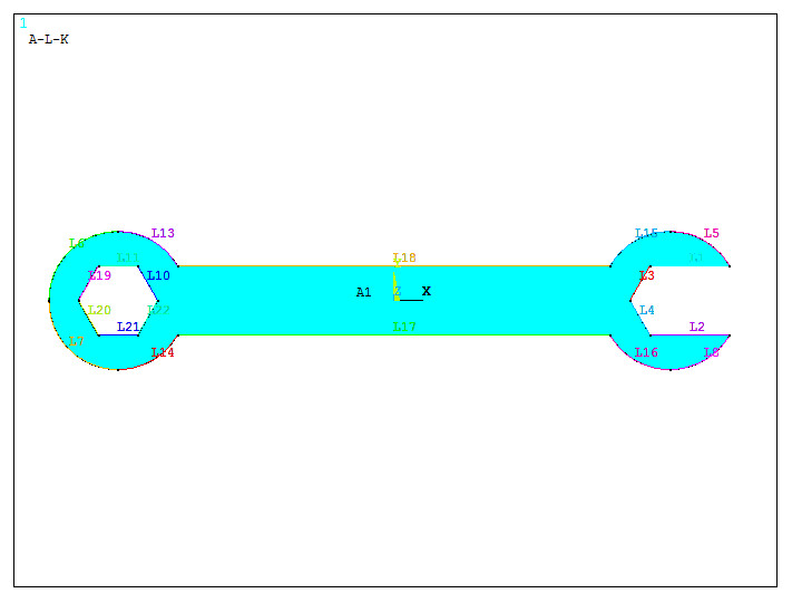
Figure 30. Numbering Lines and Areas.
Finally, create the radius of curvature with the "Line Fillet" option.
Main Menu > Preprocessor > Modeling > Create > Lines > Line Fillet
Create these lines according to Figure 31. After each "Line Fillet" operation, click "Apply" and "OK".
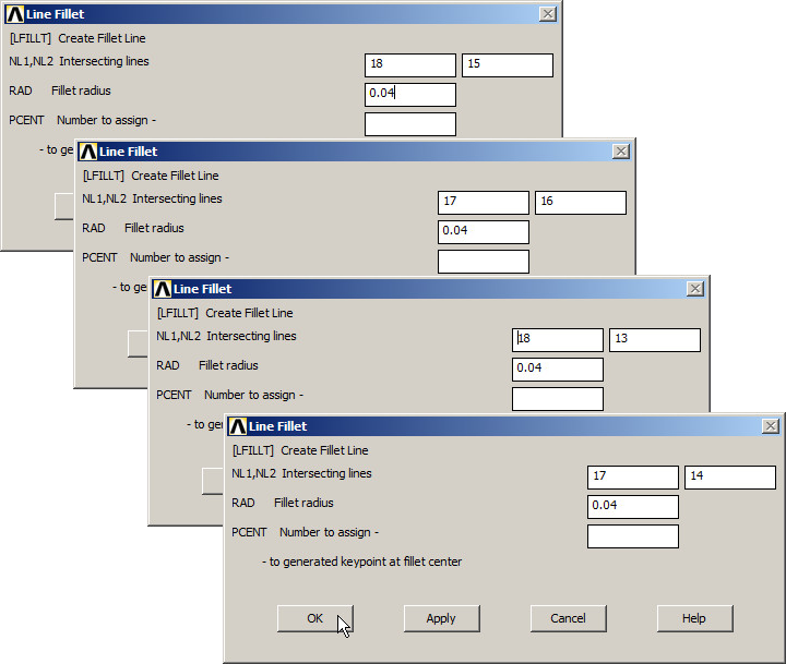
Figure 31. "Line Fillet" operation.
Figure 32 shows the new lines to define the curvature.
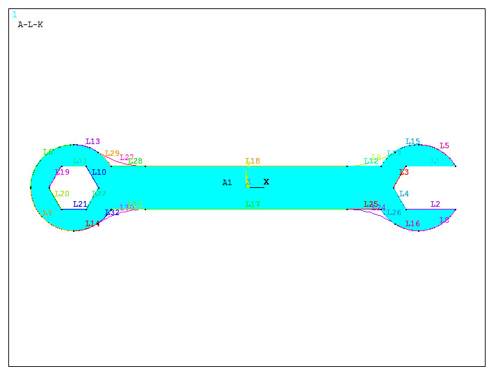
Figure 32. Lines for the curvature.
Create the areas defined by these lines.
Main Menu > Preprocessor > Modeling > Create > Areas > Arbitrary > By Lines
Selecting three lines in the corresponding parts of the model, four new areas are created (Figure 33).
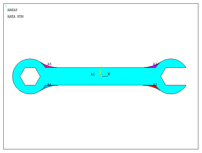
Figure 33. Creating areas.
Finally, "Add Areas" to complete the model (Figure 34).
Figure 34. Model with the new areas.
The geometry is completely defined. Now, define an element size for the meshing process. As indicated in Figure 35, the size for the element is 0.002 m.
Main Menu > Preprocessor > Meshing > Size Cntrls > ManualSize > Areas > All Areas
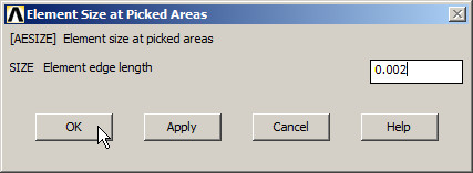
Figure 35. Element size for the meshing process.
Finish the meshing process:
Main Menu > Preprocessor > Meshing > Mesh > Areas > Free
Figure 36 shows the meshed model.
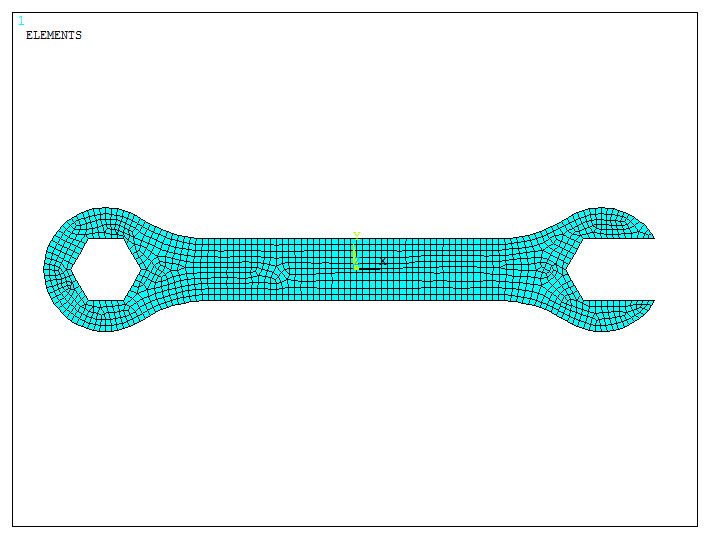
Figure 36. Meshed model.
LOADS AND BOUNDARY CONDITIONS
For the boundary conditions, the hexagonal hole at the left is considered fixed. So, all degrees of freedom have to be restricted on the lines that define the hexagon.
Main Menu > Preprocessor > Loads > Define Loads > Apply > Structural > Displacement > On Lines
Select the six lines and "All DOF" (Figure 37).
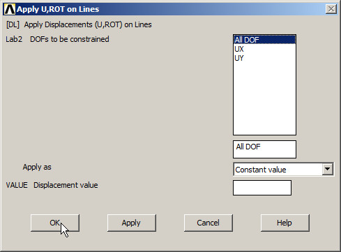
Figure 37. "All DOF" on the lines that define the hexagonal hole.
On the other hand, a force of 1000 N acts at the tangent point between the top line of the rectangle and the line that defines the radius of curvature at the right side:
Main Menu > Preprocessor > Loads > Define Loads > Apply > Structural > Force/Moment > On Keypoints
Input this force in FY direction as indicated in Figure 38.
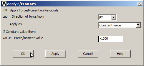
Figure 38. Applying 1000 N in FY direction.
Figure 39 displays graphically the meshed model with the load and boundary conditions.
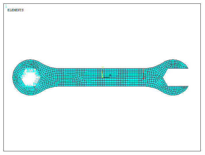
Figure 39. Meshed model with the boundary conditions.
SOLUTION
Solve the problem:
Main Menu > Solution > Solve > Current LS
"Solution is done!".
RESULTS
Plot the stress distribution and the deformed model (Figure 40):
Main Menu > General Postproc > Plot Results > Contour Plot > Nodal Solu
Select "Stress – von Mises stress" in "Contour Nodal Solution Data". And "Deformed shape with undeformed model" in "Undisplaced shape key".
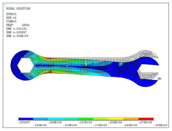
Figure 40. Stress distribution in the wrench.
The maximum value of the stress is 0.309·109 Pa. In case that the allowable stress is 260 MPa, there is a graphical option to evaluate the parts of the model that exceed the allowable stress.
Activate the option "Uniform Contours" (Figure 41):
Utility Menu > PlotCtrls > Style > Contours > Uniform Contours
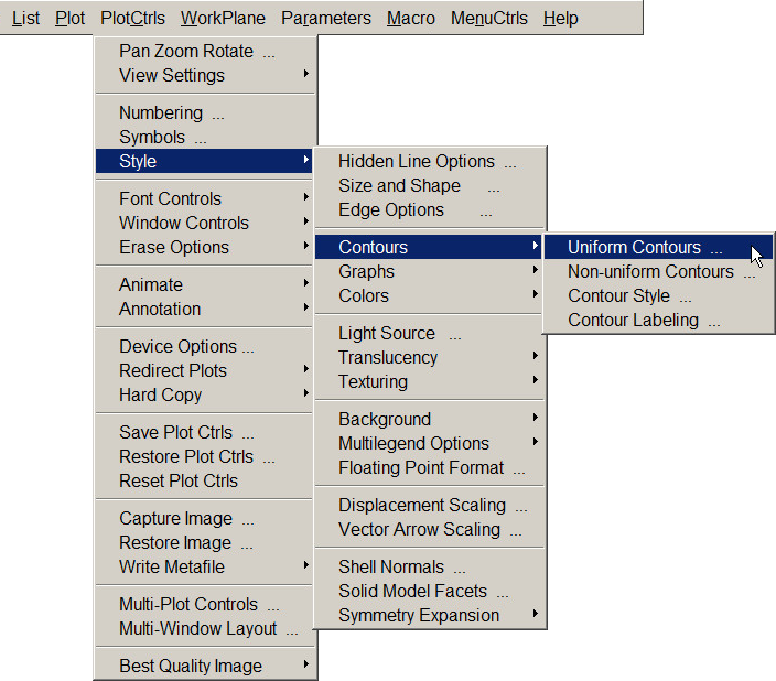
Figure 41. "Uniform Contours" option.
As indicated in Figure 42, select "User specified intervals" and define the minimum and maximum values for the stress.
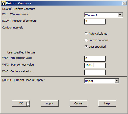
Figure 42. Defining the minimum and maximum values for the stress.
Click "OK". The parts of the model that exceed the defined range for the stress are displayed in grey colour (Figure 43).
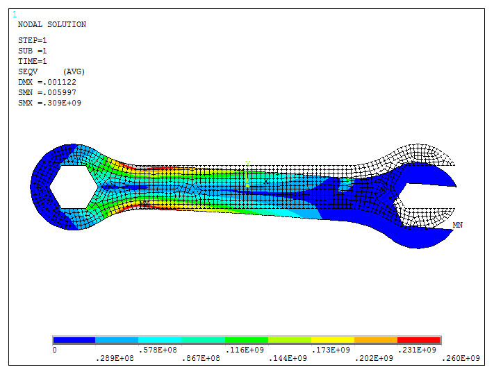
Figure 43. "Von Mises Stress".