PROBLEM
Figure 1 represents a tensile-test specimen. The material for this specimen is Nylon 6.6 and supports an axial load.
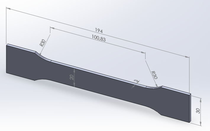
Figure 1. Tensile-test specimen.
Determine the stress distribution in the specimen and the maximum value of the load required for not exceeding the yield stress. Table 1 shows the mechanical properties of the Nylon 6.6.
Table 1. Material properties.
| Nylon 6.6 | |
| Enylon 6.6 | 2200 N/mm2 |
| Sy nylon 6.6 | 72 N/mm2 |
| νnylon 6.6 | 0.28 |
GEOMETRY OF THE MODEL
First, define a name for the problem: "tensile-test specimen".
Utility Menu > File > Change Title
And define the problem as "Structural".
Main Menu > Preferences
Y se activa "Structural".
For this particular problem, select the element type "Solid 8 node 183", which is a plane element (Figure 2):
Main Menu > Preprocessor > Element Type > Add/Edit/Delete
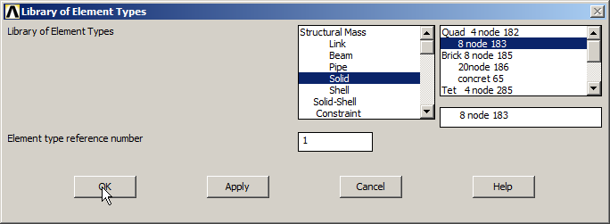
Figure 2. Element Type.
In "Options" select "Plane strs w/thk" to define the thickness (Figure 3):
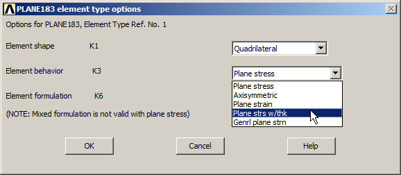
Figure 3. Plane stress with thickness.
The thickness is 3 mm, as indicated in Figure 4:
Main Menu > Preprocessor > Real Constants > Add/Edit/Delete
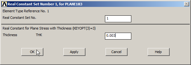
Figure 4. Thickness 3 mm.
Input the material properties (Figure 5):
Main Menu > Preprocessor > Material Props > Material Models
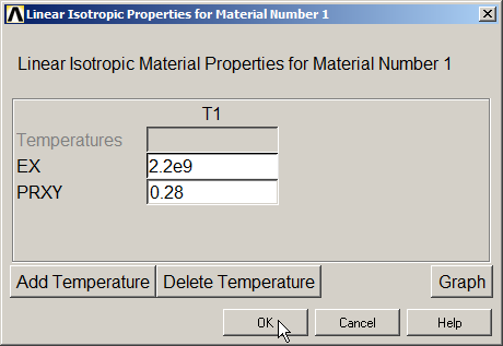
Figure 5. Mechanical properties for the material.
Now define the geometry of the model by creating two rectangular areas, as indicated in Table 2. Figure 6 shows the process to create these two rectangular areas.
Table 2. Rectangular areas (mm).
| X1 | X2 | Y1 | Y2 | |
| Rectángulo 1 | 0 | 97 | 0 | 10 |
| Rectángulo 2 | 50.415 | 97 | 0 | 15 |
Main Menu > Preprocessor > Modeling > Create > Areas > Rectangle > By Dimensions
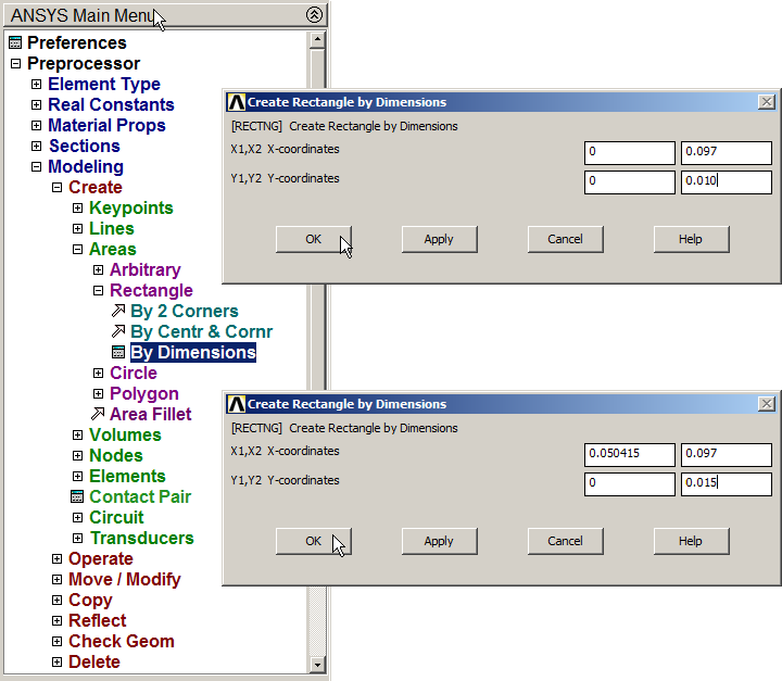
Figure 6. Creating two rectangular areas.
Next, create a circular area to define the radius of curvature, as indicated in Figure 7.
Main Menu > Preprocessor > Modeling > Create > Areas > Circle > Solid Circle
Table 3 shows the coordinates for this circular area.
Table 3. Circular area (mm).
| X | Y | Radio | |
| Círculo | 50.415 | 40 | 30 |
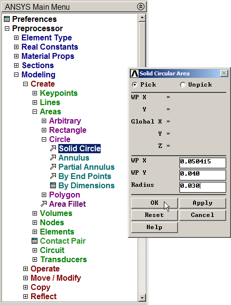
Figure 7. Circular area.
The three areas are displayed graphically in Figure 8.
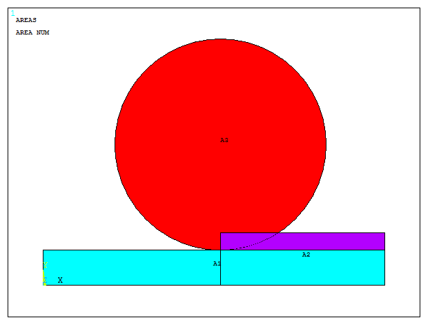
Figure 8. Created areas.
Now, number the areas (Figure 9):
Utility Menu > PlotCtrls > Numbering
And click "On " in "AREAS".
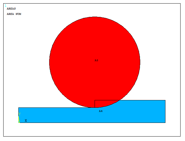
Figure 9. Numbering areas.
Next, subtract the contact area between the circle and the rectangles.
Main Menu > Preprocessor > Modeling > Operate > Booleans > Subtract > Areas
Select the three areas, click "OK" and then select the circular area and "OK".
Now, add the areas.
Main Menu > Preprocessor > Modeling > Operate > Booleans > Add > Areas
And click "Pick All".
Figure 10 represents the area after "Subtract" operation.
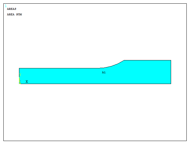
Figure 10. Created area after "Subtract" and "Add" operations.
Copy this area to complete the geometry. This step is done by "Reflect Areas" option, as indicated in Figure 11.
Main Menu > Preprocessor > Modeling > Reflect > Areas
Click "X-Z plane Y" for the first copy. Then, repeat this operation with the new area for "Y-Z plane X".
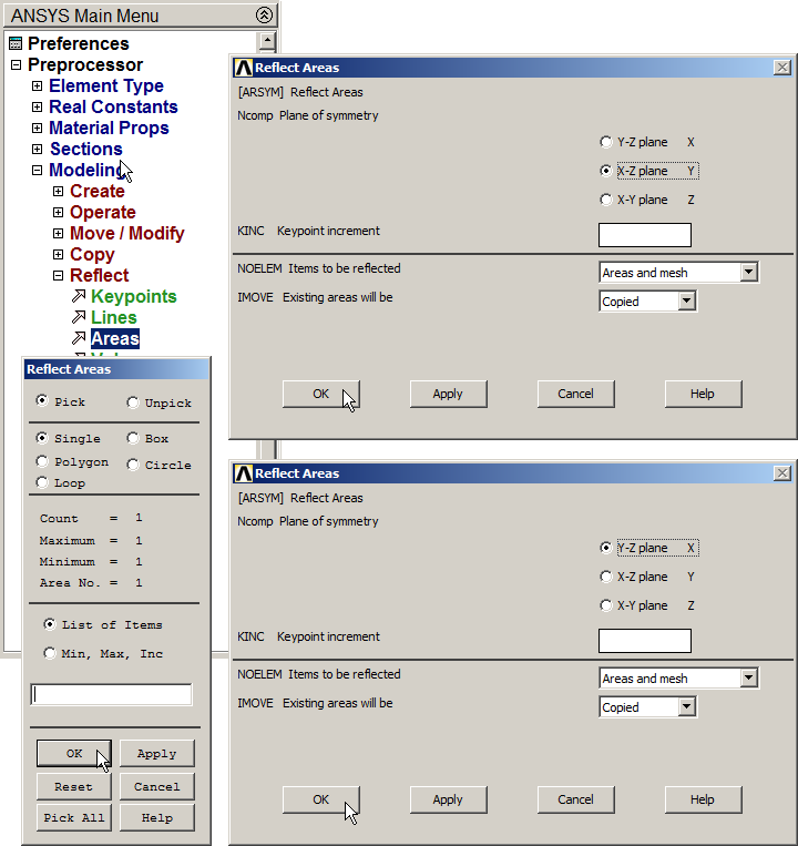
Figure 11. "Reflect Areas" operation.
Figure 12 displays graphically the model after "Reflect Areas" operation.
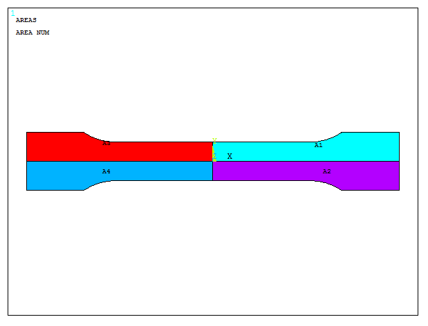
Figure 12. Areas for the tensile-test specimen model.
Finally, add the areas.
Main Menu > Preprocessor > Modeling > Operate > Booleans > Add > Areas
Click "Pick All". Figure 13 shows the complete model for the tensile-test specimen.
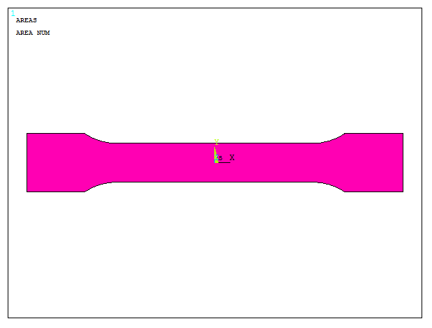
Figure 13. Complete model for the tensile-test specimen.
Now, define the working plane (Figure 14).
Utility Menu > WorkPlane > Display Working Plane
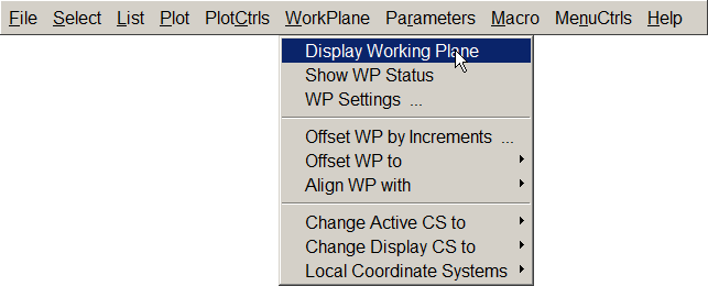
Figure 14. "Display Working Plane".
For the working plane, input the parameters indicated in Figure 15.
Utility Menu > WorkPlane > WP Settings
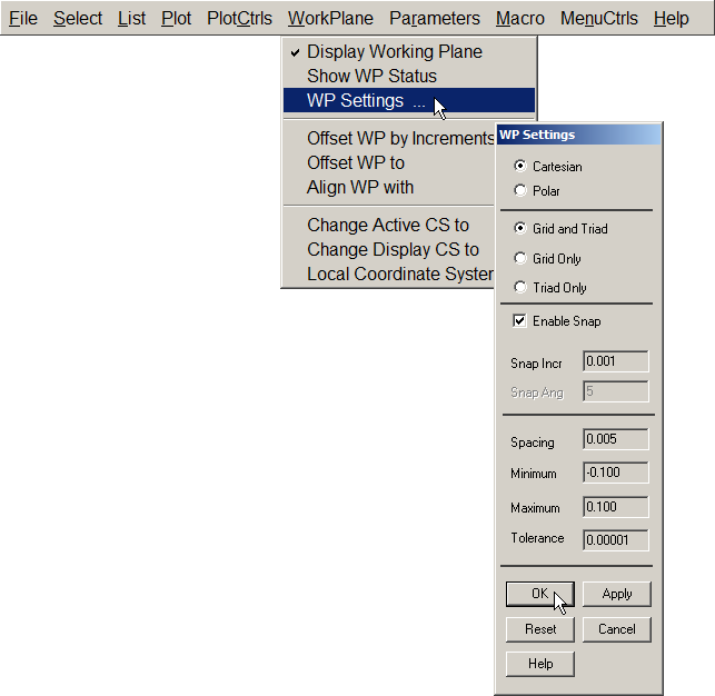
Figure 15. "Working Plane Settings".
Input 1 mm in "Snap Incr" so that the cursor moves with this increment.
The grid spacing on the screen is 5 mm (Spacing). The work area is defined between the minimum value of -0.1 m and the maximum value of 0.1 m.
Next, input 90º for "Offset WP by Increments" to rotate the working plane as indicated in Figure 16.
Utility Menu > WorkPlane > Offset WP by Increments
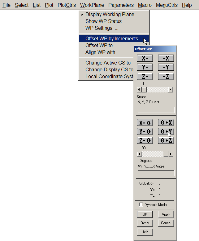
Figure 16. "Offset Working Plane by Increments".
Now, repeat the option "Offset WP by Increments" to move the plane 77 mm to the right and divide areas by working plane (Figure 17).
Main Menu > Preprocessor > Modeling > Operate > Booleans > Divide > Area by WrkPlane
Click "Pick All".
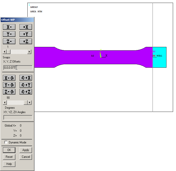
Figure 17. Divide area by Working Plane (right side).
Again use "Offset WP by Increments" to move the plane 154 mm to the left and divide areas (Figure 18).
Main Menu > Preprocessor > Modeling > Operate > Booleans > Divide > Area by WrkPlane
Click "Pick All".
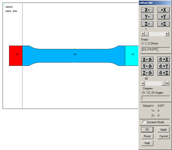
Figure 18. Divide area by Working Plane (left side).
When the geometry has been defined, mesh the model.
Main Menu > Preprocessor > Meshing > Size Cntrls > ManualSize > Areas > All Areas
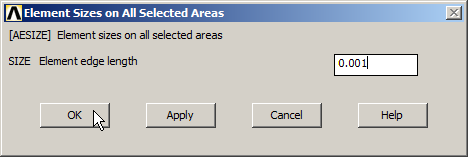
Figure 19. Element size for the mesh.
Finish the meshing process.
Main Menu > Preprocessor > Meshing > Mesh > Areas > Free
And click "Pick All". Figure 20 displays graphically the meshed model.
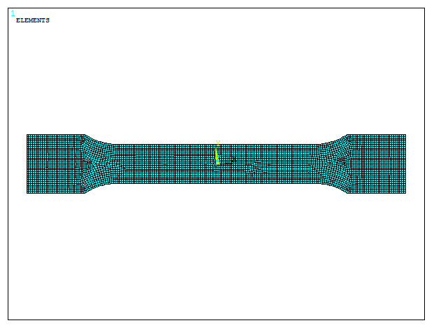
Figure 20. Meshed model.
LOADS AND BOUNDARY CONDITIONS
For the boundary conditions, restrict the displacements in UX direction at the left end, simulating the effect of the gripping jaws (Figure 21).
Main Menu > Preprocessor > Loads > Define Loads > Apply > Structural > Displacement > On Areas
And select the area at the left side.

Figure 21. Restrict the displacement in UX direction at the left side.
Now, restrict the displacement in UY direction on a keypoint (Figure 22).
Main Menu > Preprocessor > Loads > Define Loads > Apply > Structural > Displacement > On Keypoints
And select the keypoint located at the bottom left.
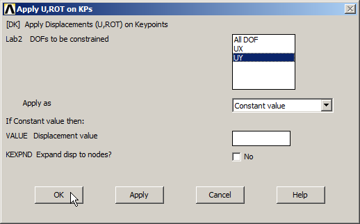
Figure 22. Restrict displacement in UY direction.
And a displacement of 5 mm in UX direction is set at the right end, as indicated in Figure 23.
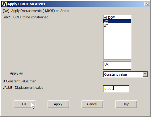
Figure 23. Restrict displacement in UX direction (5 mm).
Figure 24 represents the tensile-test specimen with the boundary conditions.
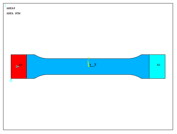
Figure 24. Geometric model with the boundary conditions.
SOLUTION
Solve the problem.
Main Menu > Solution > Solve > Current LS
"Solution is done!".
RESULTS
First, evaluate the deformation of the model (Figure 25).
Main Menu > General Postproc > Plot Results > Deformed Shape
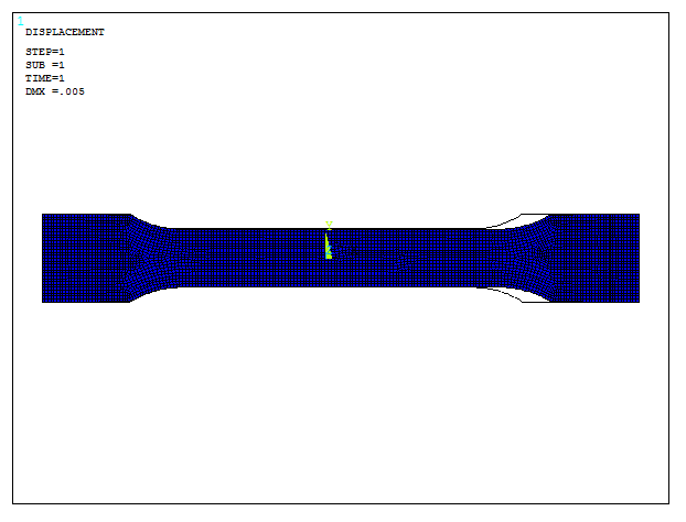
Figure 25. Deformed model.
For the stress distribution (Figure 26):
Main Menu > General Postproc > Plot Results > Contour Plot > Nodal Solu
And select "von Mises stress".

Figure 26. Stress distribution in the model.
Considering that the yield stress for this material is 72 MPa, adjust the maximum displacement. From the obtained results, the new value of the displacement is (72/90.6)*0.005, as indicated in Figure 27.
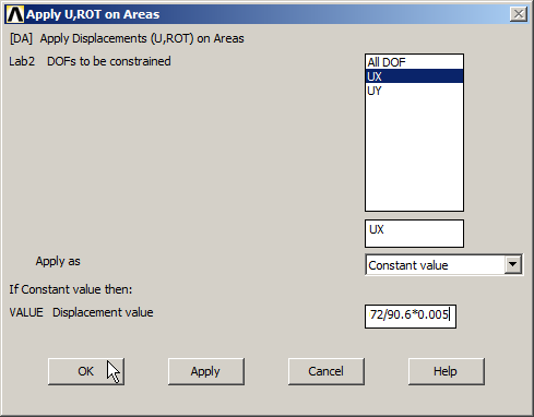
Figure 27. New restriction for the displacement in UX direction.
Solve the problem to obtain the new stress distribution (Figure 28). So, the maximum displacement can be set in 3.974 mm without exceeding the elastic limit.
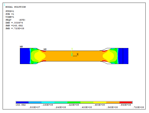
Figure 28. Deformation restricted by the yield stress.
Finally, list the values of the reactions on the right area. First select this area:
Utility Menu > Select > Entities
Then define "Areas" and click "OK". After that, select "Nodes – Attached to – Areas", as indicated in Figure 29.
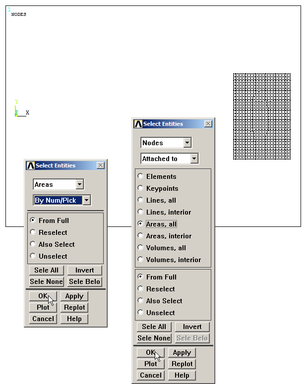
Figure 29. Selecting the area.
Figure 30 lists the reactions on the selected nodes. So, the total value is the maximum load that can be applied for not exceeding the yield stress.
Main Menu > General Postproc > List Results > Reaction Solu
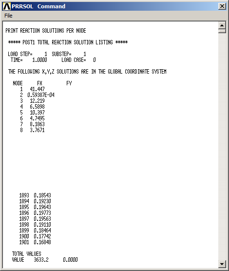
Figure 30. List of the reactions on the selected nodes.